where the derivative of solutions depends only on \(x\) (the dependent variable) is called an autonomous equation. If we think of \(t\) as time, the naming comes from the fact that the equation is independent of time.
We return to the cooling coffee problem (Example 1.3.5). Newton’s law of cooling says
\begin{equation*}
\frac{dx}{dt} = k (A-x) ,
\end{equation*}
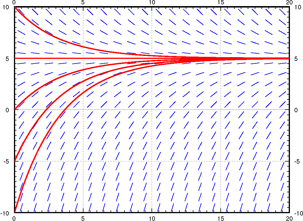
where \(x\) is the temperature, \(t\) is time, \(k\) is some positive constant, and \(A\) is the ambient temperature. See Figure 1.3.6 for an example with \(k=0.3\) and \(A=5\text{.}\)
Note the solution \(x(t)=A\) (in the figure \(x=5\)). We call these constant solutions the equilibrium solutions. The points on the \(x\)-axis where \(f(x) = 0\) are called critical points of the differential equation (1.7.1). The point \(x=A\) is a critical point. In fact, each critical point corresponds to an equilibrium solution.
Now, we want to determine what happens for other values of \(x\) that are not \(A\text{.}\) Based on the existence and uniqueness theorem in Section 1.5 for first order differential equations, the fact that \(k(A-x)\) and its partial derivative in \(x\text{,}\)\(-k\text{,}\) are continuous everywhere gives that solution curves can not cross. This means that since we know \(x(t)=A\) is a solution, if a solution starts below \(x(t)=A\text{,}\) it must always stay there, and solutions that start above \(x(t)=A\) will also stay there. For more information about what the solutions do, we’ll need to look back at the equation and some sample solution curves.
Note also, by looking at the graph, that the solution \(x=A\) is stable in that small perturbations in \(x\) do not lead to substantially different solutions as \(t\) grows. If we change the initial condition a little bit, then as \(t \to \infty\) we get \(x(t) \to A\text{.}\) We call such a critical point asymptotically stable. In this simple example, it turns out that all solutions in fact go to \(A\) as \(t \to \infty\text{.}\) If there is a critical point where all nearby solutions move away from the critical point, we say it is unstable. If some nearby solutions go towards the critical point, and some others move away, then we say it is semistable. The final option is that solutions nearby neither move towards nor away from the critical point, and these critical points are called stable.
The last of these options may seem strange at first, and that is because stable critical points are not possible for autonomous equations with one unknown function. If a solution does not move towards or away from a critical point, that means it doesn’t move anywhere, and so is a critical point on its own. However, when we get to autonomous systems in Section 4.7 and Section 5.1, we will see that in two dimensions, this is possible (think of a circle that does not spiral into or away from the center point).
A graph showing several solution curves, including one that is a horizontal line at \(5\text{.}\) All of the solution curves exponentially approach \(5\) as \(t \rightarrow \infty\text{.}\)
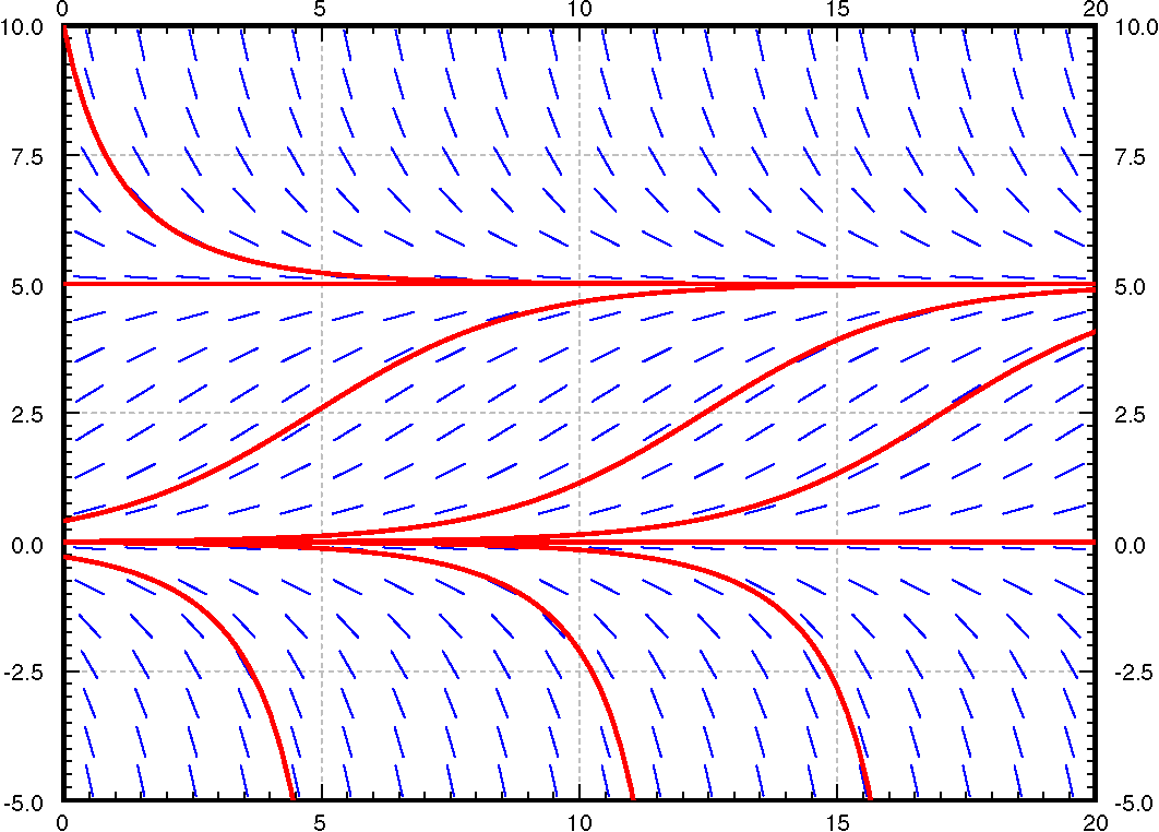
A graph showing several solution curves, including horizontal lines at \(0\) and \(5\text{.}\) The solutions that start below zero head downward off the edge of the graph. The solutions that start between \(0\) and \(5\text{,}\) as well as the ones that start above \(5\text{,}\) converge to \(5\) as \(t \rightarrow \infty\text{.}\)
for some positive \(k\) and \(M\text{.}\) This equation is commonly used to model population if we know the limiting population \(M\text{,}\) that is the maximum sustainable population. The logistic equation leads to less catastrophic predictions on world population than \(x'=kx\text{.}\) In the real world there is no such thing as negative population, but we will still consider negative \(x\) for the purposes of the math.
See Figure 1.7.2(b) for an example, \(x' = 0.1 x(5-x)\text{.}\) There are two critical points, \(x=0\) and \(x=5\text{.}\) The critical point at \(x=5\) is asymptotically stable, while the critical point at \(x=0\) is unstable.
It is not necessary to find the exact solutions to talk about the long term behavior of the solutions. From the slope field above of \(x' = 0.1 x(5-x)\text{,}\) we see that
Here DNE means “does not exist”. From just looking at the slope field we cannot quite decide what happens if \(x(0) < 0\text{.}\) It could be that the solution does not exist for \(t\) all the way to \(\infty\text{.}\) Think of the equation \(x' = x^2\text{;}\) we have seen that solutions only exist for some finite period of time. Same can happen here. In our example equation above it turns out that the solution does not exist for all time, but to see that we would have to solve the equation. In any case, the solution does go to \(-\infty\text{,}\) but it may get there rather quickly.
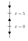
If we are interested only in the long term behavior of the solution, we would be doing unnecessary work if we solved the equation exactly. We could draw the slope field, but it is easier to just look at the phase diagram or phase line, which is a simple way to visualize the behavior of autonomous equations. The phase line for this equation is visible in Figure 1.7.3. In this case there is one dependent variable \(x\text{.}\) We draw the \(x\)-axis, we mark all the critical points, and then we draw arrows in between. Since \(x\) is the dependent variable we draw the axis vertically, as it appears in the slope field diagrams above. If \(f(x) > 0\text{,}\) we draw an up arrow. If \(f(x) < 0\text{,}\) we draw a down arrow. To figure this out, we could just plug in some \(x\) between the critical points, \(f(x)\) will have the same sign at all \(x\) between two critical points as long \(f(x)\) is continuous. For example, \(f(6) = -0.6 < 0\text{,}\) so \(f(x) < 0\) for \(x > 5\text{,}\) and the arrow above \(x=5\) is a down arrow. Next, \(f(1) = 0.4 > 0\text{,}\) so \(f(x) > 0\) whenever \(0 < x < 5\text{,}\) and the arrow points up. Finally, \(f(-1) = -0.6 < 0\) so \(f(x) < 0\) when \(x <
0\text{,}\) and the arrow points down.
Armed with the phase diagram, it is easy to sketch the solutions approximately: As time \(t\) moves from left to right, the graph of a solution goes up if the arrow is up, and it goes down if the arrow is down.
Try sketching a few solutions simply from looking at the phase diagram. Check with the preceding graphs to see if you are getting the types of curves that match the solutions.
Once we draw the phase diagram, we can use it to classify critical points as asymptotically stable, semistable, or unstable based on whether the “arrows” point into or away from the critical point on each side. Two arrows in means that the critical point is asymptotically stable, two arrows away means unstable, and one in one out means semistable.
Find all equilibrium solutions for this equation, and determine their stability. Draw a phase line and use this information to sketch some approximate solution curves.
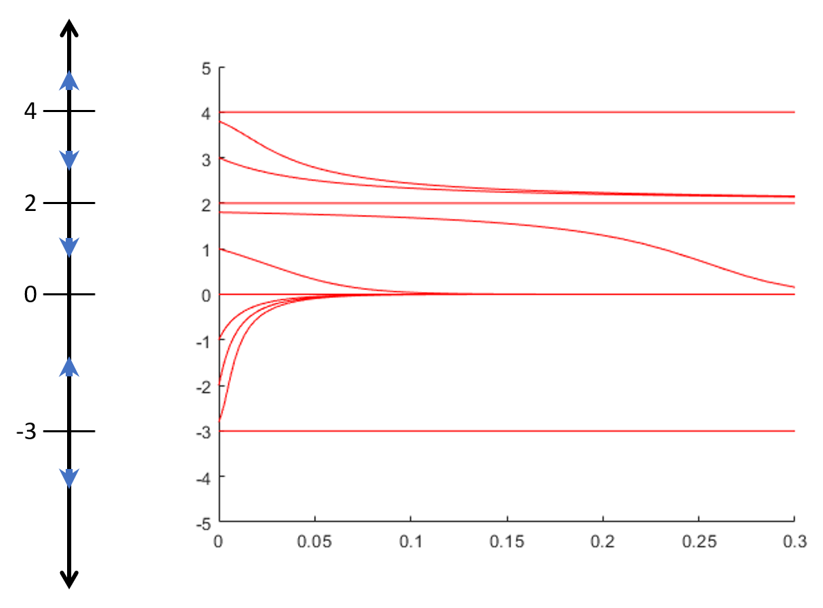
This equation is already in factored form. This makes it simple to determine the equilibrium solutions as \(x=0\text{,}\)\(x=2\text{,}\)\(x=-3\) and \(x=4\text{.}\) In order to determine the stability of each critical point and draw the phase line, we need to plug in values surrounding these points to \(f(x) = x(x-2)^2(x+3)(x-4)\text{.}\) We can see that
This lets us draw the phase line and determine the stability of each critical point. Thus, we see that \(x=-3\) is an unstable critical point, \(x=0\) is asymptotically stable, \(x=2\) is semistable, and \(x=4\) is unstable. A set of sample solution curves also validates these conclusions.
A two-part plot showing a phase line on the left side and a sketch of solution curves on the right. The phase line shows that 4 is unstable, 2 is semistable, 0 is asymptotically stable, and -3 is unstable. The solution curve sketches also show this, with graphs converging to 0 and converging to 2 from above.
We can tell from the phase line for an autonomous equation when the solution will be increasing or decreasing. Is there any more we can learn about the shape of these graphs? There is, and it comes from looking for the concavity, which is determined by the second derivative.
So, the solution is concave up if \(f'(x)f(x)\) is positive, and concave down if that is negative. Phrased another way, the solution is concave up if \(f\) and \(f'\) have the same sign, and it is concave down if \(f\) and \(f'\) have opposite signs.
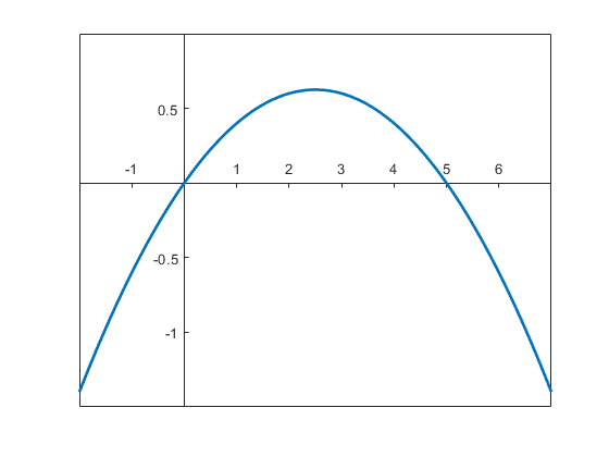
Let’s see what this looks like in action. Take the logistic equation \(x' = 0.1x(5-x)\text{,}\) whose solutions are plotted in Figure 1.7.2(b). Figure 1.7.7(a) shows the graph of \(f(x)\) as a function of \(x\) for this scenario. When do \(f\) and \(f'\) have the same sign? Well, this happens when \(f\) is both positive and increasing, or negative and decreasing. This happens between \(0\) and the vertex, as well as for \(x> 5\text{.}\) The vertex here is at \(x=2.5\text{,}\) and so we conlude that the solution should be concave up when \(x\) is on the intervals \((0, 2.5)\) and \((5, \infty)\text{,}\) and be concave down otherwise. Looking back at Figure 1.7.2(b), this is exactly what we observe. All of the solutions between \(0\) and \(5\) seem to “flip over” to be concave down when \(x\) crosses \(2.5\text{.}\)
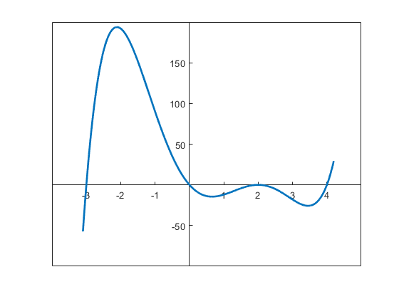
The graph of a high degree polynomial that starts by increasing through the first root at \(-3\text{.}\) It has other roots at \(0\text{,}\) a double root at \(2\text{,}\) and a root at \(4\text{.}\)
The same can be seen for solutions to (1.7.2), even though we can’t compute the extreme values explicitly. Figure 1.7.7(b) shows the graph of \(f(x)\) vs. \(x\) for this situation. Between each pair of equilibrium solutions there is a critical point of \(f\) (in the Calculus 1 sense) where the derivative is zero, and at this point, the derivative changes sign, and since the function value does not change sign, the concavity of the solution to the differential equation flips at this point. Comparing this graph and these points where concavity shifts with the solutions drawn in Figure 1.7.6 again validates these results.
Draw the phase diagram for \(-4\pi \leq x \leq 4\pi\text{.}\) On this interval mark the critical points asymptotically stable, semistable, or unstable.
Let \(y' = (y-2)(y^2 + 1)(y+3)\text{.}\) Sketch a phase diagram for this differential equation. Find and classify all critical points. If \(y(0) = 0\text{,}\) what will happen to the solution as \(t \rightarrow \infty\text{?}\)
Let \(y' = (y-3)(y+2)^2e^y\text{.}\) Sketch a phase diagram for this differential equation. Find and classify all critical points. If \(y(0) = 0\text{,}\) what will happen to the solution as \(t \rightarrow \infty\text{?}\)
Consider the DE \(\dfrac{dy}{dt}=y^5-3y^4+3y^3-y^2\text{.}\) Find and classify all equilibrium solutions of this DE. Then sketch a representative selection of solution curves.
Suppose \(\frac{dx}{dt} = (x-\alpha)(x-\beta)\) for two numbers \(\alpha <
\beta\text{.}\) In parts b), c), and d), find \(\displaystyle \lim_{t\to\infty} x(t)\) based on the phase diagram.
A disease is spreading through the country. Let \(x\) be the number of people infected. Let the constant \(S\) be the number of people susceptible to infection. The infection rate \(\frac{dx}{dt}\) is proportional to the product of already infected people, \(x\text{,}\) and the number of susceptible but uninfected people, \(S-x\text{.}\)