As we said, the general first order equation we are studying looks like
\begin{equation*}
y' = f(x,y).
\end{equation*}
A lot of the time, we cannot simply solve these kinds of equations explicitly, because our direct integration method only works when the equation is of the form \(y' = f(x),\) which we could integrate directly. In these more complicated cases, it would be nice if we could at least figure out the shape and behavior of the solutions, or find approximate solutions.
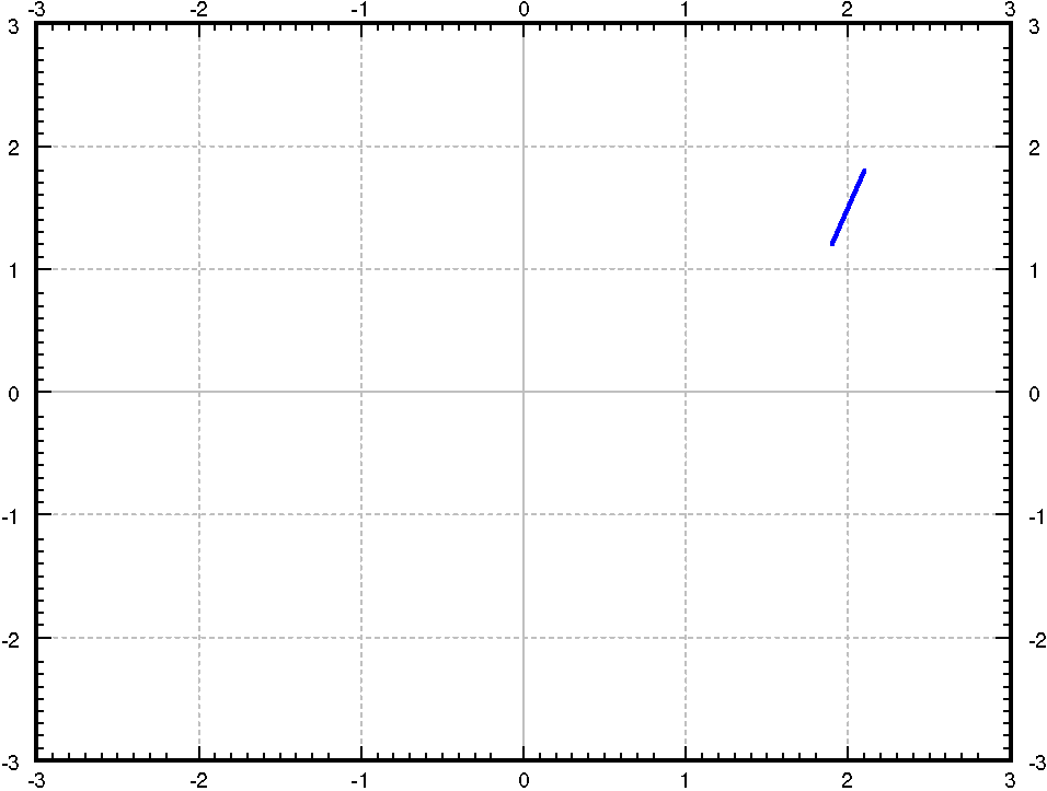
Suppose that we have a solution to the equation \(y' = f(x,y)\) with \(y(x_0) = y_0\text{.}\) What does the fact that this solves the differential equation tell us about the solution? It tells us that the derivative of the solution at this point will be \(f(x_0, y_0)\text{.}\) Graphically, the derivative gives the slope of the solution, so it means that the solution will pass through the point \((x_0, y_0)\) and will have slope \(f(x_0, y_0)\text{.}\) For example, if \(f(x,y) = xy\text{,}\) then at point \((2,1.5)\) we draw a short line of slope \(xy = 2 \times 1.5 = 3\text{.}\) So, if \(y(x)\) is a solution and \(y(2) = 1.5\text{,}\) then the equation mandates that \(y'(2) = 3\text{.}\) See Figure 1.2.1.
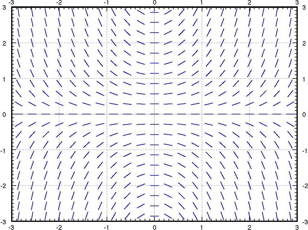
To get an idea of how solutions behave, we draw such lines at lots of points in the plane, not just the point \((2,1.5)\text{.}\) We would ideally want to see the slope at every point, but that is just not possible. Usually we pick a grid of points fine enough so that it shows the behavior, but not too fine so that we can still recognize the individual lines. We call this picture the slope field of the equation. See Figure 1.2.2(a) for the slope field of the equation \(y' = xy\text{.}\) Usually in practice, one does not do this by hand, but has a computer do the drawing.
The idea of a slope field is that it tells us how the graph of the solution should be sloped, or should curve, if it passed through a given point. Having a wide variety of slopes plotted in our slope field gives an idea of how all of the solutions behave for a bunch of different initial conditions. Which curve we want in particular, and where we should start the curve, depends on the initial condition.
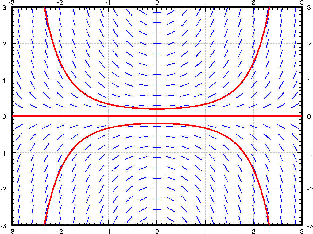
Suppose we are given a specific initial condition \(y(x_0) = y_0\text{.}\) A solution, that is, the graph of the solution, would be a curve that follows the slopes we drew, starting from the point \((x_0, y_0)\text{.}\) For a few sample solutions, see Figure 1.2.2(b). It is easy to roughly sketch (or at least imagine) possible solutions in the slope field, just from looking at the slope field itself. You simply sketch a line that roughly fits the little line segments and goes through your initial condition. The graph should “flow” along the little slopes that are on the slope field.
A graph showing many short lines, the slope of which is \(xy\) at the point \((x,y)\text{.}\) On top of this are three red curves that follow the slope field lines given. Above the horizontal axis, the graph is somewhat parabolic facing upwards. Another red line is straight across the horizontal axis. The graph below the horizontal axis is somewhat like a downward facing parabola.
By looking at the slope field we get a lot of information about the behavior of solutions without having to solve the equation. For example, in Figure 1.2.2(b) we see what the solutions do when the initial conditions are \(y(0) > 0\text{,}\)\(y(0) = 0\) and \(y(0) < 0\text{.}\) A small change in the initial condition causes quite different behavior. We see this behavior just from the slope field and imagining what solutions ought to do.
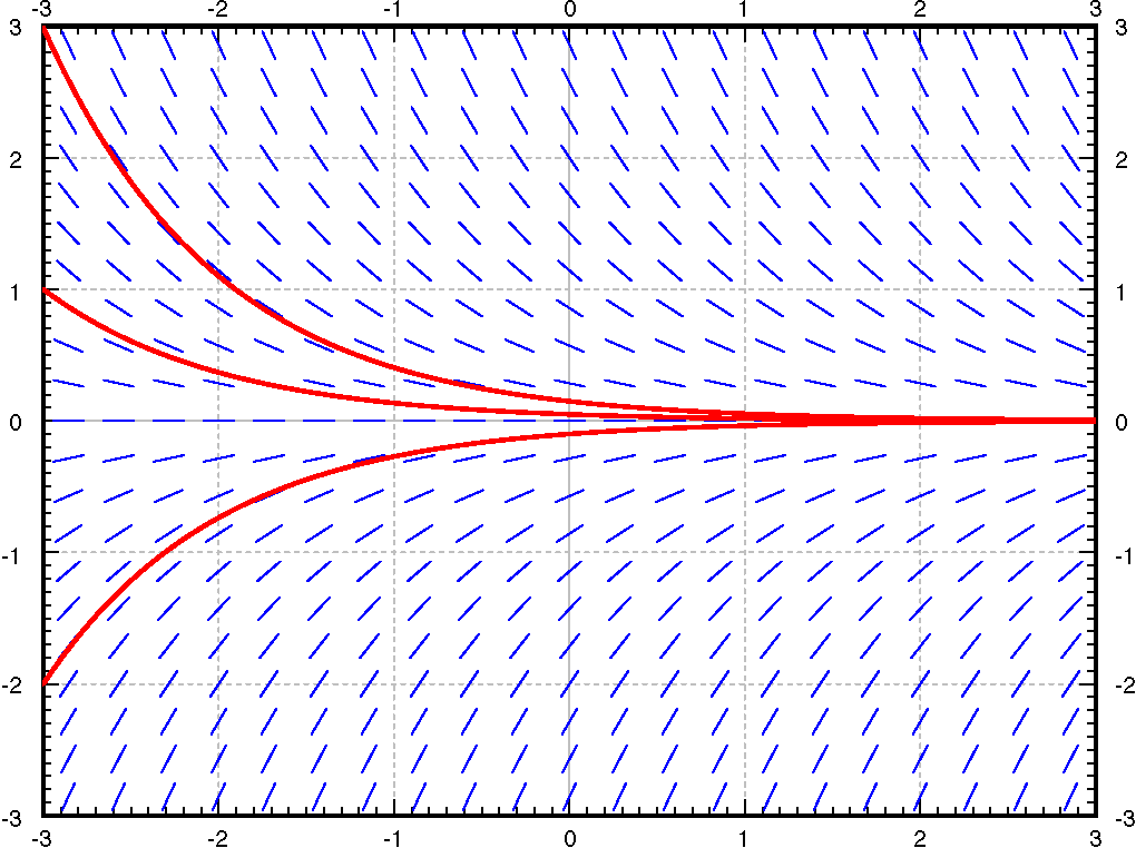
We see a different behavior for the equation \(y' = -y\text{.}\) The slope field and a few solutions is in Figure 1.2.3 . If we think of moving from left to right (perhaps \(x\) is time and time is usually increasing), then we see that no matter what \(y(0)\) is, all solutions tend to zero as \(x\) tends to infinity. Again that behavior is clear from simply looking at the slope field itself.
A graph showing sloped lines that all point towards the horizontal axis, getting flatter as they get closer to that axis. A few red solution lines are drawn on top of this that all converge to zero as the graph goes to the right.
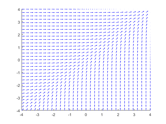
Sketch slope field for \(y'=e^{x-y}\text{.}\) How do the solutions behave as \(x\) grows? Can you guess a particular solution by looking at the slope field?
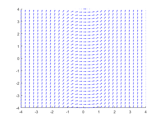
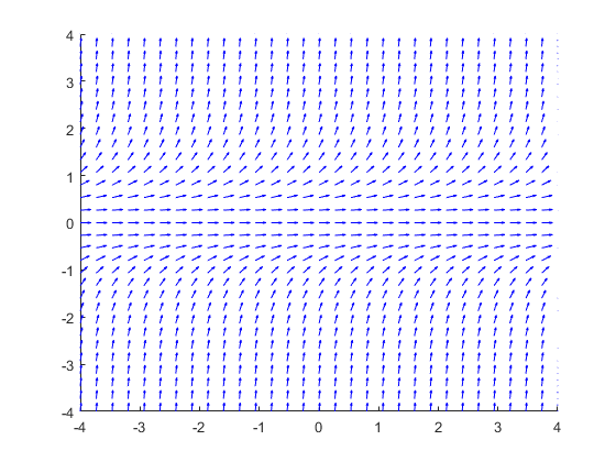
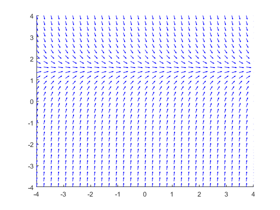
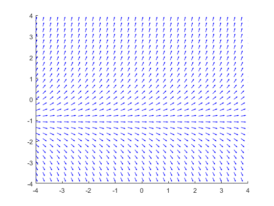
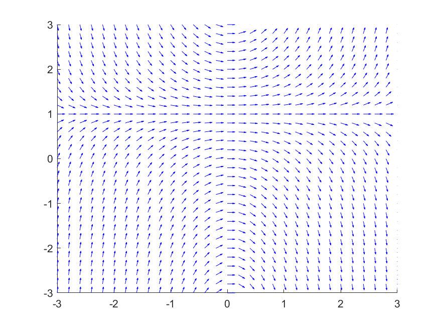
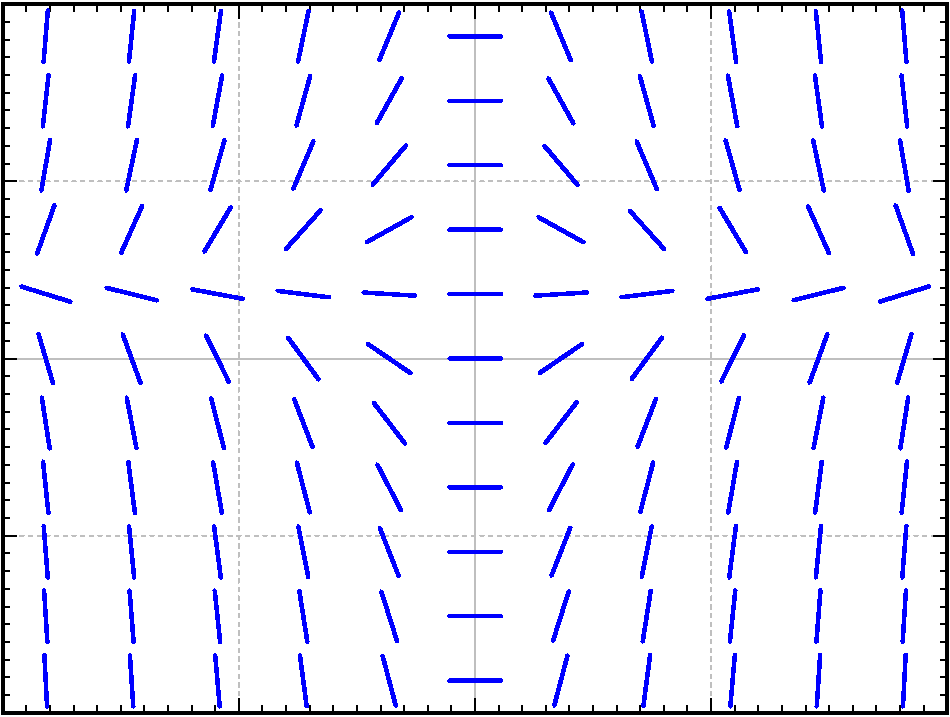
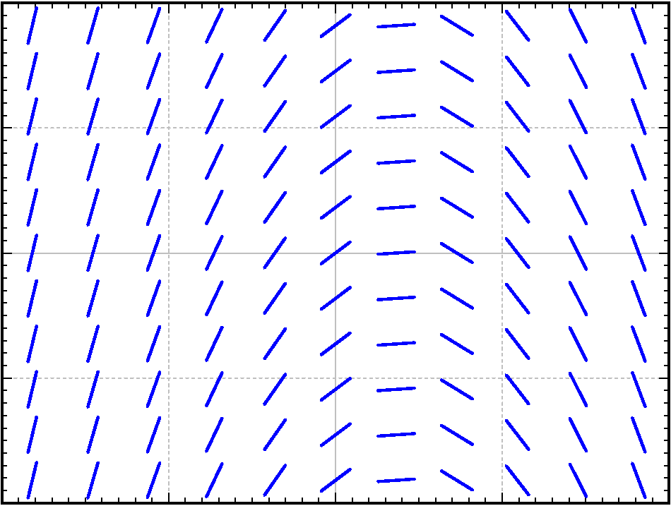
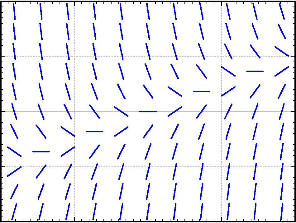
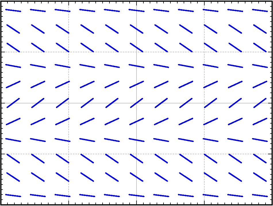
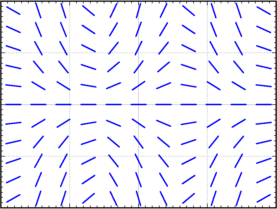
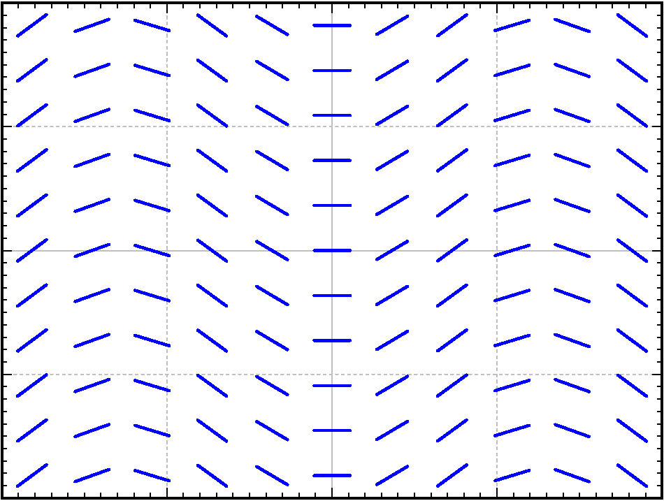
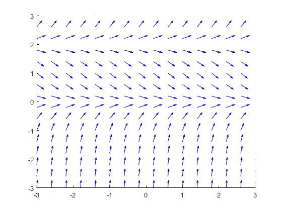
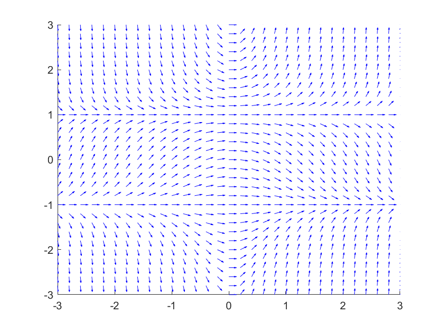
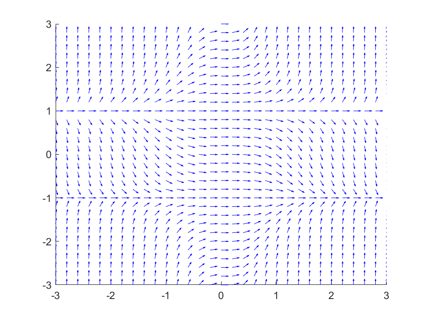
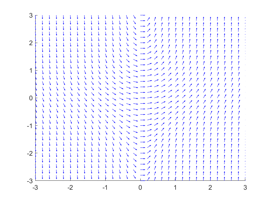
For each of the following differential equations, sketch out a slope field on \(-3 < x < 3\) and \(-3 < y < 3\) and determine the overall behavior of the solutions to the equation as \(t \rightarrow \infty\text{.}\) If this fact depends on the value of the solution at \(t=0\text{,}\) explain how it changes.
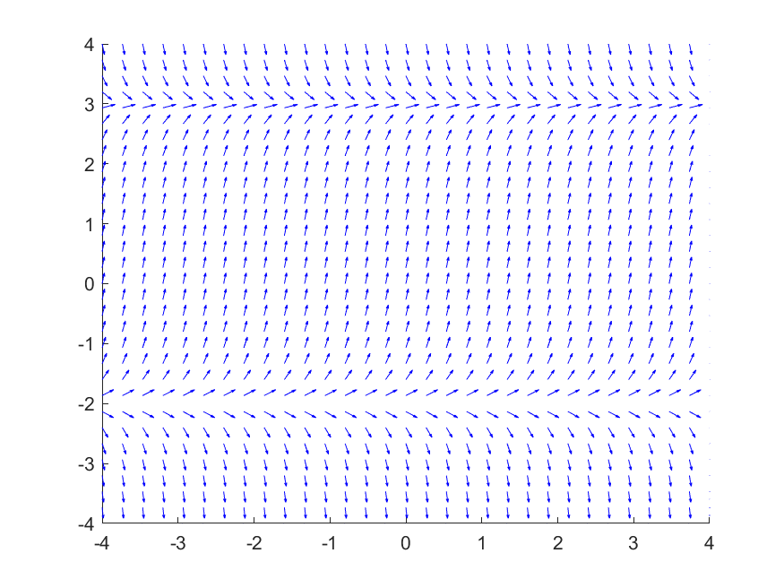
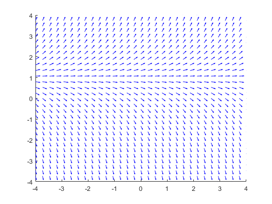
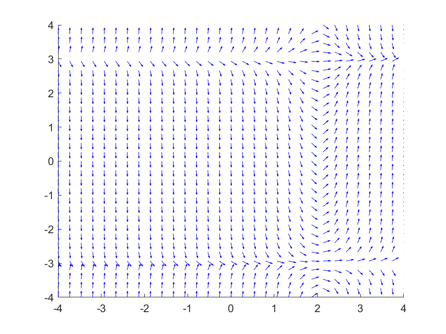
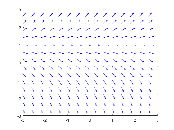
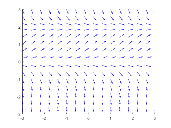
The slope field for the differential equation \(y' = (3-y)(y+2)\) is below. If we find the solution to this differential equation with initial condition, \(y(0) = 1\text{,}\) what will happen to the solution as \(t \rightarrow \infty\text{?}\) Use the slope field and your knowledge of the equation to determine the long-time behavior of this solution.
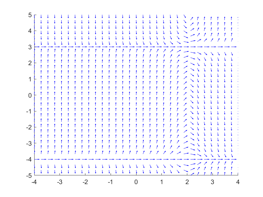
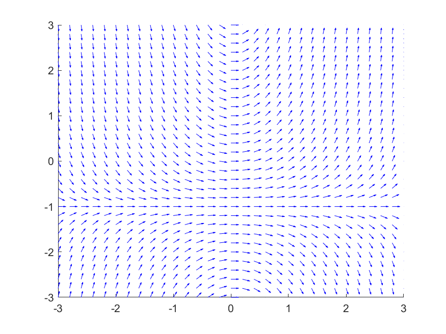
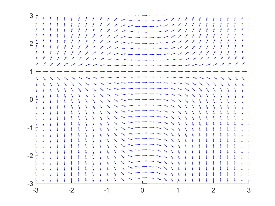
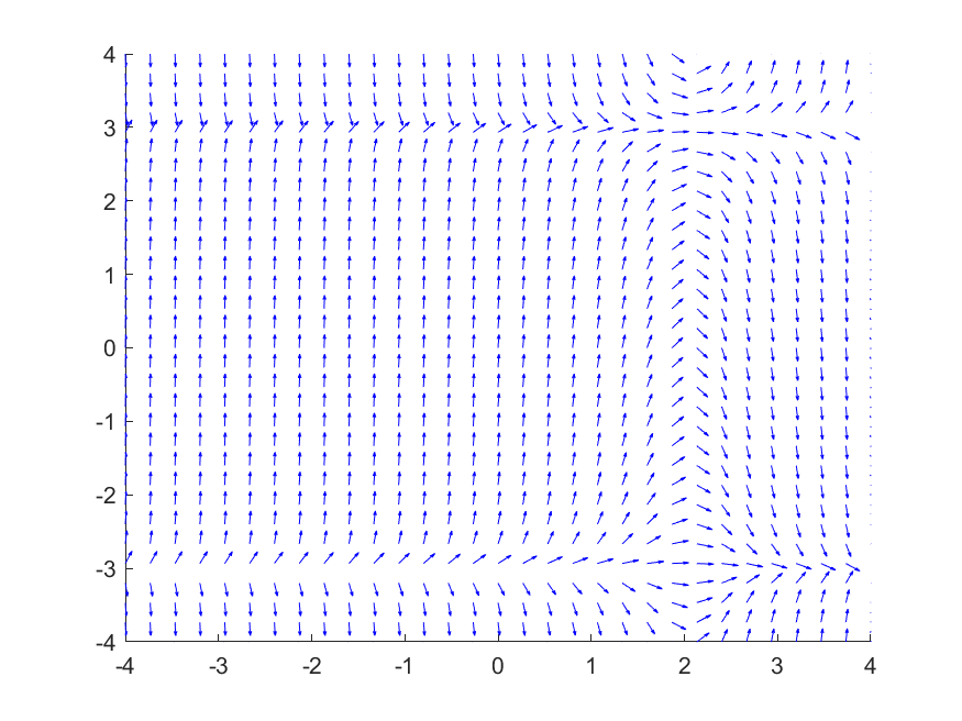
The slope field for the differential equation \(y' = (t-2)(y+4)(y-3)\) is below. If we find the solution to this differential equation with initial condition, \(y(0) = 1\text{,}\) what will happen to the solution as \(t \rightarrow \infty\text{?}\) Use the slope field and your knowledge of the equation to determine the long-time behavior of this solution.
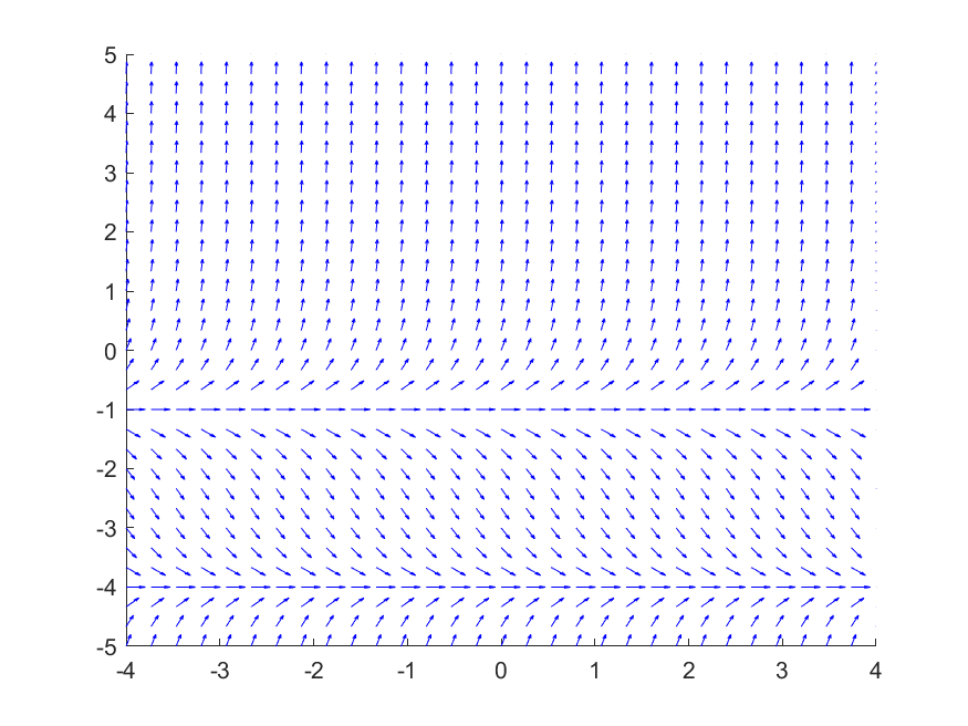
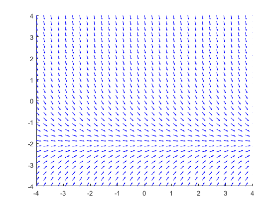
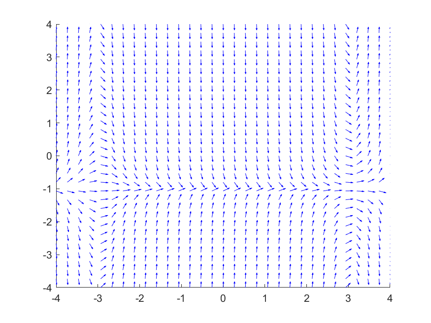
The slope field for the differential equation \(y' = (y+1)(y+4)\) is below. If we find the solution to this differential equation with initial condition, \(y(0) = 1\text{,}\) what will happen to the solution as \(t \rightarrow \infty\text{?}\) Use the slope field and your knowledge of the equation to determine the long-time behavior of this solution.
Take \(y' = f(x,y)\text{,}\)\(y(0) = 0\text{,}\) where \(f(x,y) > 1\) for all \(x\) and \(y\text{.}\) If the solution exists for all \(x\text{,}\) can you say what happens to \(y(x)\) as \(x\) goes to positive infinity? Explain.
Describe what each of the following facts about the function \(f(x,y)\) tells you about the slope field for the differential equation \(y' = f(x,y)\text{.}\)