Determinant

Section 3.4 Determinant

Objectives

After this section, you will be able to:

Compute the determinant of a $2\times 2$ matrix,
🔗

🔗
Use cofactor expansion to compute the determinant of larger matrices, and
🔗

🔗
Use the determinant to make statements about invertibility or linear independence of the columns of that matrix.
🔗

🔗

For square matrices we define a useful quantity called the determinant. We define the determinant of a $1 \times 1$ matrix as the value of its only entry

\begin{equation*} \det \left( \begin{bmatrix} a \end{bmatrix} \right) \overset{\text{def}}{=} a . \end{equation*}

For a $2 \times 2$ matrix we define

\begin{equation*} \det \left( \begin{bmatrix} a & b \\ c & d \end{bmatrix} \right) \overset{\text{def}}{=} ad-bc . \end{equation*}

🔗

Before defining the determinant for larger matrices, we note the meaning of the determinant. An $n \times n$ matrix gives a mapping of the $n$-dimensional euclidean space ${\mathbb{R}}^n$ to itself. In particular, a $2 \times 2$ matrix $A$ is a mapping of the plane to itself. The determinant of $A$ is the factor by which the area of objects changes. If we take the unit square (square of side 1) in the plane, then $A$ takes the square to a parallelogram of area $\lvert\det(A)\rvert\text{.}$ The sign of $\det(A)$ denotes a change of orientation (negative if the axes get flipped). For example, let

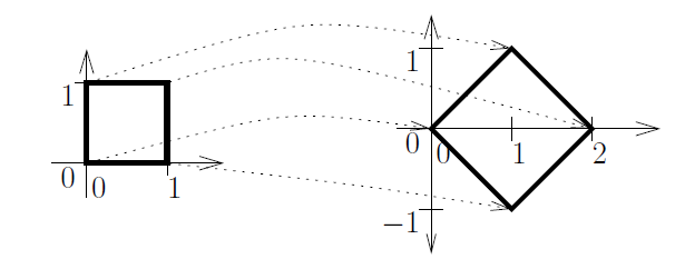
\begin{equation*} A = \begin{bmatrix} 1 & 1 \\ -1 & 1 \end{bmatrix} . \end{equation*}

Then $\det(A) = 1+1 = 2\text{.}$ Let us see where $A$ sends the unit square with vertices $(0,0)\text{,}$ $(1,0)\text{,}$ $(0,1)\text{,}$ and $(1,1)\text{.}$ The point $(0,0)$ gets sent to $(0,0)\text{.}$

\begin{equation*} \begin{bmatrix} 1 & 1 \\ -1 & 1 \end{bmatrix} \begin{bmatrix} 1 \\ 0 \end{bmatrix} = \begin{bmatrix} 1 \\ -1 \end{bmatrix} , \qquad \begin{bmatrix} 1 & 1 \\ -1 & 1 \end{bmatrix} \begin{bmatrix} 0 \\ 1 \end{bmatrix} = \begin{bmatrix} 1 \\ 1 \end{bmatrix} , \qquad \begin{bmatrix} 1 & 1 \\ -1 & 1 \end{bmatrix} \begin{bmatrix} 1 \\ 1 \end{bmatrix} = \begin{bmatrix} 2 \\ 0 \end{bmatrix} . \end{equation*}

The image of the square is another square with vertices $(0,0)\text{,}$ $(1,-1)\text{,}$ $(1,1)\text{,}$ and $(2,0)\text{.}$ The image square has a side of length $\sqrt{2}$ and is therefore of area 2. See Figure 3.4.1.

🔗

ALT TEXT HERE — Figure 3.4.1. Image of the unit quare via the mapping $A\text{.}$
🔗

In general the image of a square is going to be a paralellogram. In high school geometry, you may have seen a formula for computing the area of a parallelogram with vertices $(0,0)\text{,}$ $(a,c)\text{,}$ $(b,d)$ and $(a+b,c+d)\text{.}$ The area is

\begin{equation*} \left\lvert \, \det \left( \begin{bmatrix} a & b \\ c & d \end{bmatrix} \right) \, \right\lvert = \lvert a d - b c \rvert . \end{equation*}

The vertical lines above mean absolute value. The matrix $\left[ \begin{smallmatrix} a & b \\ c & d \end{smallmatrix} \right]$ carries the unit square to the given parallelogram.

🔗

There are a number of ways to define the determinant for an $n \times n$ matrix. Let us use the so-called cofactor expansion. We define $A_{ij}$ as the matrix $A$ with the $i^{\text{th}}$ row and the $j^{\text{th}}$ column deleted. For example,

\begin{equation*} \text{If} \qquad A = \begin{bmatrix} 1 & 2 & 3 \\ 4 & 5 & 6 \\ 7 & 8 & 9 \end{bmatrix} , \qquad \text{then} \qquad A_{12} = \begin{bmatrix} 4 & 6 \\ 7 & 9 \end{bmatrix} \qquad \text{and} \qquad A_{23} = \begin{bmatrix} 1 & 2 \\ 7 & 8 \end{bmatrix} . \end{equation*}

We now define the determinant recursively

\begin{equation*} \det (A) \overset{\text{def}}{=} \sum_{j=1}^n {(-1)}^{1+j} a_{1j} \det (A_{1j}) , \end{equation*}

or in other words

\begin{equation*} \det (A) = a_{11} \det (A_{11}) - a_{12} \det (A_{12}) + a_{13} \det (A_{13}) - \cdots \begin{cases} + a_{1n} \det (A_{1n}) & \text{if } n \text{ is odd,} \\ - a_{1n} \det (A_{1n}) & \text{if } n \text{ even.} \end{cases} \end{equation*}

For a $3 \times 3$ matrix, we get

\begin{equation*} \det (A) = a_{11} \det (A_{11}) - a_{12} \det (A_{12}) + a_{13} \det (A_{13})\text{.} \end{equation*}

For example,

\begin{align*} \det \left( \begin{bmatrix} 1 & 2 & 3 \\ 4 & 5 & 6 \\ 7 & 8 & 9 \end{bmatrix} \right) \amp = 1 \cdot \det \left( \begin{bmatrix} 5 & 6 \\ 8 & 9 \end{bmatrix} \right) - 2 \cdot \det \left( \begin{bmatrix} 4 & 6 \\ 7 & 9 \end{bmatrix} \right) + 3 \cdot \det \left( \begin{bmatrix} 4 & 5 \\ 7 & 8 \end{bmatrix} \right) \\ \amp = 1 (5 \cdot 9 - 6 \cdot 8) - 2 (4 \cdot 9 - 6 \cdot 7) + 3 (4 \cdot 8 - 5 \cdot 7) = 0\text{.} \end{align*}

🔗

It turns out that we did not have to necessarily use the first row. That is for any $i\text{,}$

\begin{equation*} \det (A) = \sum_{j=1}^n {(-1)}^{i+j} a_{ij} \det (A_{ij}) . \end{equation*}

It is sometimes useful to use a row other than the first. In the following example it is more convenient to expand along the second row. Notice that for the second row we are starting with a negative sign.

\begin{align*} \det \left( \begin{bmatrix} 1 & 2 & 3 \\ 0 & 5 & 0 \\ 7 & 8 & 9 \end{bmatrix} \right) \amp = - 0 \cdot \det \left( \begin{bmatrix} 2 & 3 \\ 8 & 9 \end{bmatrix} \right) + 5 \cdot \det \left( \begin{bmatrix} 1 & 3 \\ 7 & 9 \end{bmatrix} \right) - 0 \cdot \det \left( \begin{bmatrix} 1 & 2 \\ 7 & 8 \end{bmatrix} \right) \\ \amp = 0 + 5 (1 \cdot 9 - 3 \cdot 7) + 0 = -60\text{.} \end{align*}

Let us check if it is really the same as expanding along the first row,

\begin{align*} \det \left( \begin{bmatrix} 1 & 2 & 3 \\ 0 & 5 & 0 \\ 7 & 8 & 9 \end{bmatrix} \right) \amp = 1 \cdot \det \left( \begin{bmatrix} 5 & 0 \\ 8 & 9 \end{bmatrix} \right) - 2 \cdot \det \left( \begin{bmatrix} 0 & 0 \\ 7 & 9 \end{bmatrix} \right) + 3 \cdot \det \left( \begin{bmatrix} 0 & 5 \\ 7 & 8 \end{bmatrix} \right) \\ \amp = 1 (5 \cdot 9 - 0 \cdot 8) - 2 (0 \cdot 9 - 0 \cdot 7) + 3 (0 \cdot 8 - 5 \cdot 7) = -60\text{.} \end{align*}

🔗

In computing the determinant, we alternately add and subtract the determinants of the submatrices $A_{ij}$ multiplied by $a_{ij}$ for a fixed $i$ and all $j\text{.}$ The numbers ${(-1)}^{i+j}\det(A_{ij})$ are called cofactors of the matrix. And that is why this method of computing the determinant is called the cofactor expansion.

🔗

Similarly we do not need to expand along a row, we can expand along a column. For any $j$

\begin{equation*} \det (A) = \sum_{i=1}^n {(-1)}^{i+j} a_{ij} \det (A_{ij}) . \end{equation*}

A related fact is that

\begin{equation*} \det (A) = \det (A^T) . \end{equation*}

🔗

Recall that a matrix is upper triangular if all elements below the main diagonal are 0. For example,

\begin{equation*} \begin{bmatrix} 1 & 2 & 3 \\ 0 & 5 & 6 \\ 0 & 0 & 9 \end{bmatrix} \end{equation*}

is upper triangular. Similarly a lower triangular matrix is one where everything above the diagonal is zero. For example,

\begin{equation*} \begin{bmatrix} 1 & 0 & 0 \\ 4 & 5 & 0 \\ 7 & 8 & 9 \end{bmatrix} . \end{equation*}

🔗

The determinant for triangular matrices is very simple to compute. Consider the lower triangular matrix. If we expand along the first row, we find that the determinant is 1 times the determinant of the lower triangular matrix $\left[ \begin{smallmatrix} 5 & 0 \\ 8 & 9 \end{smallmatrix} \right]\text{.}$ So the deteriminant is just the product of the diagonal entries:

\begin{equation*} \det \left( \begin{bmatrix} 1 & 0 & 0 \\ 4 & 5 & 0 \\ 7 & 8 & 9 \end{bmatrix} \right) = 1 \cdot 5 \cdot 9 = 45 . \end{equation*}

Similarly for upper triangular matrices

\begin{equation*} \det \left( \begin{bmatrix} 1 & 2 & 3 \\ 0 & 5 & 6 \\ 0 & 0 & 9 \end{bmatrix} \right) = 1 \cdot 5 \cdot 9 = 45 . \end{equation*}

In general, if $A$ is triangular, then

\begin{equation*} \det (A) = a_{11} a_{22} \cdots a_{nn} . \end{equation*}

🔗

If $A$ is diagonal, then it is also triangular (upper and lower), so same formula applies. For example,

\begin{equation*} \det \left( \begin{bmatrix} 2 & 0 & 0 \\ 0 & 3 & 0 \\ 0 & 0 & 5 \end{bmatrix} \right) = 2 \cdot 3 \cdot 5 = 30 . \end{equation*}

🔗

In particular, the identity matrix $I$ is diagonal, and the diagonal entries are all 1. Thus,

\begin{equation*} \det(I) = 1 . \end{equation*}

🔗

Another way that we can compute determinants is by using row reduction. Since the row echelon form is a diagonal matrix, this will make it easy to compute the determinant using the product of the diagonal entries. However, we need to know how the determinant is affected by elementary row operations.

🔗

Theorem 3.4.2. Determinants and Elementary Row Operations.

Let $A$ be a square $n\times n$ matrix.

If $B$ obtained from $A$ by interchanging two rows (or two columns) of $A\text{,}$ then $\det(B) = -\det(A)\text{.}$
🔗

🔗
If $B$ is obtained from $A$ by multiplying a row of column by the number $r\text{,}$ then $\det(B) = r\det(A)\text{.}$
🔗

🔗
If $B$ is obtained from $A$ by multiplying a row (or column) by a non-zero number $r$ and adding the result to another row, then $\det(B) = \det(A)\text{.}$
🔗

🔗

🔗

Proof.

The proof of each of these facts comes from the cofactor expansion of the determinant.

Assume that $B$ is obtained by interchanging the first and second row of $A\text{.}$ We will use cofactor expansion along the first row to find the determinant of $A\text{,}$ and the second row for the determinant of $B\text{.}$ We get that

\begin{equation*} \det(A) = \sum_{j=1}^n (-1)^{1+j}a_{1j} \det(A_{1j}) \end{equation*}

and

\begin{equation*} \det(B) = \sum_{j=1}^n (-1)^{2+j}b_{2j} \det(B_{2j}). \end{equation*}

However, since the second row of $B$ is the first row of $A\text{,}$ we know that $b_{2j} = a_{1j}$ for all $j\text{.}$ In addition, this swap means that we also have that $B_{2j} = A_{1j}$ for each of the cofactors in this expansion. All of these cofactor matrices are made up of the second through last rows of $A\text{,}$ with the appropriate columns removed at each step.

🔗

Therefore, the only difference between these two formulas is that the $A$ formula starts with $(-1)^{1+j}$ and the $B$ formula starts with $(-1)^{2+j}\text{.}$ Thus, $\det(B)$ will have an additional factor of $-1$ in it, giving the desired result.
🔗

The exact same process works for swapping any two adjacent rows of the matrix, giving that this also provides a $-1$ in the computation of the determinant. For non-adjacent rows, we use the fact that to any swap of non-adjacent rows of a matrix requires an odd number of adjacent row swaps. For example, if we want to swap rows $1$ and $3\text{,}$ we can swap row 1 with row 2, then row 2 with row 3, and finally swap row 1 with row 2 again. This will put the first row in the third spot and the third row up in the first slot. Since each of these adjacent switches adds a minus sign, doing an odd number of switches still results in adding a single minus sign to the computation of the determinant.
🔗

🔗
Assume that we want to multiply the $k$th row of $A$ by the number $r$ to get $B\text{.}$ We use cofactor expansion along this same $k$th row to find the determinant of each matrix. We get that

\begin{equation*} \det(A) = \sum_{j=1}^n (-1)^{k+j}a_{kj}\det(A_{kj}) \end{equation*}

and

\begin{equation*} \det(B) = \sum_{j=1}^n (-1)^{k+j}b_{kj}\det(B_{kj}) = \sum_{j=1}^n (-1)^{k+j}ra_{kj} \det(B_{kj}). \end{equation*}

However, the minor $B_{kj}$ ignores the $k$th row of the matrix $B\text{,}$ so the minors are identical to those of $A\text{.}$ Thus, we have that

\begin{equation*} \det(B) = \sum_{j=1}^n (-1)^{k+j}ra_{kj} \det(B_{kj}) = r\sum_{j=1}^n (-1)^{k+j}a_{kj} \det(A_{kj}) = r\det(A) . \end{equation*}

🔗

🔗
Assume that $B$ is formed by adding $r$ copies of the $k$th row of $A$ to the $i$th row. Since the $i$th row is the one being changed, we will use cofactor expansion there to compute each determinant. We get that

\begin{equation*} \det(A) = \sum_{j=1}^n (-1)^{i+j}a_{ij}\det(A_{ij} \end{equation*}

and

\begin{equation*} \det(B) = \sum_{j=1}^n (-1)^{i+j} b_{ij}\det(B_{ij}) = \sum (-1)^{i+j} (a_{ij} + ra_{kj})\det(A_{ij}) \end{equation*}

where we have replaced the minors of $B$ by the minors of $A$ because they ignore the $i$th row, which is the only thing that has changed. We can now split the determinant of $B$ into two parts

\begin{equation*} \sum (-1)^{i+j} (a_{ij} + ra_{kj})\det(A_{ij}) = \sum (-1)^{i+j} a_{ij}\det(A_{ij}) + \sum (-1)^{i+j} ra_{kj}\det(A_{ij}). \end{equation*}

The first of these is the determinant of the matrix $A\text{.}$ The second is the determinant of a new matrix that we will call $C\text{.}$ $C$ is the same as the matrix $A\text{,}$ except that we have replaced the $i$th row of $A$ by $r$ times the $k$th row of $A\text{.}$ Thus, the $i$th row of this matrix $C$ is a multiple of the $k$th row. This means that the rows of $C$ are not linearly independent. By Theorem 3.4.7 coming up later (don’t worry, it does not depend on this result), this tells us that the determinant of $C$ is zero. Therefore

\begin{equation*} \det(B) = \det(A) + \det(C) = \det(A) \end{equation*}

so this operation does not change the determinant of the matrix.

🔗

🔗

🔗

These correspond to the three elementary row operations that we use to row reduce matrices. In order to use this to compute determinants, we need to keep track of each of these operations and how the determinant changes at each step.

🔗

Example 3.4.3.

Compute the determinant of the matrix

\begin{equation*} \begin{bmatrix} -4 & -2 & 4\\ -3 & -3 & 2\\ -2 &-3 & 1\end{bmatrix} \end{equation*}

using row reduction.

🔗

Solution.

We will go through the process of row reduction to find the determinant. We need to keep track of each time that we swap rows (to add a minus sign) and that we multiply a row by a constant (to factor in that constant). Throughout this process, we will use $A$ to refer to the initial matrix

\begin{equation*} A = \begin{bmatrix} -4 & -2 & 4\\ -3 & -3 & 2\\ -2 &-3 & 1\end{bmatrix} \end{equation*}

and $M$ will refer to wherever we are in the process. So we will start by dividing the first row of the matrix by $-4$

\begin{equation*} \begin{bmatrix} -4 & -2 & 4\\ -3 & -3 & 2\\ -2 &-3 & 1\end{bmatrix} \rightarrow \begin{bmatrix} 1 & 1/2 & -1\\ -3 & -3 & 2\\ -2 &-3 & 1\end{bmatrix}. \end{equation*}

Since we divided by $-4\text{,}$ Theorem 3.4.2 tells us that

\begin{equation*} \det(M) = -\frac{1}{4} \det(A). \end{equation*}

The next step of row reduction will be to use the 1 in the top left to cancel out the $-3$ and $-2$ below it. Part (c) in says that this doesn’t change the determinant. Therefore, the row reduction gives

\begin{equation*} \begin{bmatrix} 1 & 1/2 & -1\\ -3 & -3 & 2\\ -2 &-3 & 1\end{bmatrix} \rightarrow \begin{bmatrix} 1 & 1/2 & -1\\ 0 & -3/2 & -1\\ 0 & -2 & -1\end{bmatrix} \end{equation*}

and we still have that

\begin{equation*} \det(M) = -\frac{1}{4}\det(A). \end{equation*}

Next, we will multiply row $2$ by $-\frac{2}{3}\text{,}$ which gives

\begin{equation*} \begin{bmatrix} 1 & 1/2 & -1\\ 0 & -3/2 & -1\\ 0 & -2 & -1\end{bmatrix} \rightarrow \begin{bmatrix} 1 & 1/2 & -1\\ 0 & 1 & 2/3\\ 0 & -2 & -1\end{bmatrix}. \end{equation*}

Adding this in to our previous steps using Theorem 3.4.2, we get that

\begin{equation*} \det(M) = \left(-\frac{2}{3} \right) \left( -\frac{1}{4} \right) \det(A). \end{equation*}

Finally, we add two copies of row 2 to row 3, which does not change the determinant and gives the matrix

\begin{equation*} \begin{bmatrix} 1 & 1/2 & -1\\ 0 & 1 & 2/3\\ 0 & -2 & -1\end{bmatrix} \rightarrow \begin{bmatrix} 1 & 1/2 & -1\\ 0 & 1 & 2/3\\ 0 & 0 & 1/3\end{bmatrix} \end{equation*}

with

\begin{equation*} \det(M) = \left(-\frac{2}{3} \right) \left( -\frac{1}{4} \right) \det(A) . \end{equation*}

We can rearrange this expression to say that

\begin{equation*} \det(A) = 6\det(M) \end{equation*}

and we can easily compute that $\det(M) = \frac{1}{3}$ by multiplying the diagonal entries. Thus, we have that $\det(A) = 2\text{.}$

🔗

Checkpoint 3.4.4.

Compute $\det(A)$ using cofactor expansion and show that you get the same answer.

🔗

The determinant is telling you how geometric objects scale. If $B$ doubles the sizes of geometric objects and $A$ triples them, then $AB$ (which applies $B$ to an object and then it applies $A$) should make size go up by a factor of $6\text{.}$ This is true in general:

🔗

Theorem 3.4.5.

\begin{equation*} \det(AB) = \det(A)\det(B) . \end{equation*}

🔗

This property is one of the most useful, and it is employed often to actually compute determinants. A particularly interesting consequence is to note what it means for existence of inverses. Take $A$ and $B$ to be inverses, that is $AB=I\text{.}$ Then

\begin{equation*} \det(A)\det(B) = \det(AB) = \det(I) = 1 . \end{equation*}

Neither $\det(A)$ nor $\det(B)$ can be zero. This fact is an extremely useful property of the determinant, and one which is used often in this book:

🔗

Theorem 3.4.6.

An $n \times n$ matrix $A$ is invertible if and only if $\det (A) \not= 0\text{.}$

🔗

In fact, $\det(A^{-1}) \det(A) = 1$ says that

\begin{equation*} \det(A^{-1}) = \frac{1}{\det(A)}. \end{equation*}

So we know what the determinant of $A^{-1}$ is without computing $A^{-1}\text{.}$

🔗

Let us return to the formula for the inverse of a $2 \times 2$ matrix:

\begin{equation*} \begin{bmatrix} a & b \\ c & d \end{bmatrix}^{-1} = \frac{1}{ad-bc} \begin{bmatrix} d & -b \\ -c & a \end{bmatrix} . \end{equation*}

Notice the determinant of the matrix $[\begin{smallmatrix}a&b\\c&d\end{smallmatrix}]$ in the denominator of the fraction. The formula only works if the determinant is nonzero, otherwise we are dividing by zero.

🔗

A common notation for the determinant is a pair of vertical lines:

\begin{equation*} \begin{vmatrix} a & b \\ c & d \end{vmatrix} = \det \left( \begin{bmatrix} a & b \\ c & d \end{bmatrix} \right) . \end{equation*}

Personally, I find this notation confusing as vertical lines usually mean a positive quantity, while determinants can be negative. Also think about how to write the absolute value of a determinant. This notation is not used in this book.

🔗

With this discussion of determinants complete, we can now state a major theorem from linear algebra that will help us here and when we get back to solving differential equations using this linear algebra. In a full course on linear algebra, this theorem would be covered in full detail, including all of the proofs. For this introduction, we give some idea as to why everything is true here, but not all of the details.

🔗

Note: This is an example of an equivalence theorem, which is fairly common in mathematics. It means that if any one of the statements are true, then we know that all of the others are true as well. It means it’s harder to prove, but once we have such a theorem, it is very powerful in how we can use it going forward.

🔗

Theorem 3.4.7.

Let $A$ be an $n \times n$ matrix. The following are equivalent:

🔗

$A$ is invertible.
🔗

🔗
$\det(A) \neq 0\text{.}$
🔗

🔗
There is a unique solution to $A\vec{x} = \vec{b}$ for every vector $\vec{b}\text{.}$
🔗

🔗
The only solution to $A\vec{x} = \vec{0}$ is $\vec{x} = \vec{0}\text{.}$
🔗

🔗
The reduced row echelon form of $A$ is $I_n\text{,}$ the identity matrix.
🔗

🔗
The columns of $A$ are linearly independent.
🔗

🔗

🔗

Proof.

Why is all of this true? For (a) and (b), we have Theorem Theorem 3.4.6 to say that they are equivalent. For (c), if $A$ is invertible, then the unique solution to $A\vec{x} = \vec{b}$ is $\vec{x} = A^{-1}\vec{b}\text{.}$ If we take $\vec{b} = \vec{0}$ here, we get (d), that the solution is $\vec{x} = A^{-1}\vec{0} = \vec{0}\text{.}$ This means that reducing the system of equations $A\vec{x} = 0$ gives $x_1 = 0\text{,}$ $x_2 = 0\text{,}$ ..., $x_n = 0\text{,}$ which means the reduced row echelon form of $A$ is just the identity matrix, which is (e). Finally, this means that every column is a pivot column, so that all of the columns are linearly independent, giving (f).

🔗

$\begin{bmatrix} 1 & 3 \\ 2 & 1 \end{bmatrix}$

$\begin{bmatrix} 0 & 1 & 2 & 0 \\ 1 & 1 & -1 & 2 \\ 1 & 1 & 2 & 1 \\ 2 & -1 & -2 & 3 \end{bmatrix}$

🔗

Answer.

Consider the matrix

\begin{equation*} A = \begin{bmatrix} 0 & -1 & 0 \\ -5 & -4 & -5 \\ 2 & 3 & 4 \end{bmatrix}. \end{equation*}

🔗

(a)

Compute the determinant of $A$ using cofactor expansion along row 1.

🔗

Answer.

$-10$

🔗

(b)

Compute the determinant of $A$ using cofactor expansion along column 2.

🔗

Answer.

$-10$

🔗

(c)

Compute the determinant using row reduction.

🔗

Answer.

$-10$

Consider the matrix

\begin{equation*} A = \begin{bmatrix} -2 & 0 & 1 & 0 \\ 0 & -1 & 1 & -2 \\ -5 &3 & 1 & 3 \\ -3 & 4 & 1 & 3 \end{bmatrix}. \end{equation*}

🔗

(a)

Compute the determinant of $A$ using cofactor expansion along row 1.

🔗

Answer.

$6$

🔗

(b)

Compute the determinant of $A$ using cofactor expansion along column 4.

🔗

Answer.

$6$

🔗

(c)

Compute the determinant using row reduction.

🔗

Answer.

$6$

🔗

Consider the linear mapping from ${\mathbb R}^2$ to ${\mathbb R}^2$ given by the matrix $A = \left[ \begin{smallmatrix} 1 & x \\ 2 & 1 \end{smallmatrix} \right]$ for some number $x\text{.}$ You wish to make $A$ such that it doubles the area of every geometric figure. What are the possibilities for $x$ (there are two answers).

🔗

Answer.

$x = -\frac{1}{2},\ \frac{3}{2}$

🔗

Suppose $A$ and $S$ are $n \times n$ matrices, and $S$ is invertible. Suppose that $\det(A) = 3\text{.}$ Compute $\det(S^{-1}AS)$ and $\det(SAS^{-1})\text{.}$ Justify your answer using the theorems in this section.

🔗

Answer.

🔗

18.

Let $A$ be an $n \times n$ matrix such that $\det(A)=1\text{.}$ Compute $\det(x A)$ given a number $x\text{.}$[2] Hint: First try computing $\det(xI)\text{,}$ then note that $xA = (xI)A\text{.}$

🔗

Answer.

$x^n$

🔗

Prev Top Next