In this section we will learn how to solve linear homogeneous constant coefficient systems of ODEs by the eigenvalue method. Suppose we have such a system
where \(P\) is a constant square matrix. We wish to adapt the method for the single constant coefficient equation by trying the function \(e^{\lambda t}\text{.}\) However, \(\vec{x}\) is a vector. So we try \(\vec{x} = \vec{v} e^{\lambda t}\text{,}\) where \(\vec{v}\) is an arbitrary constant vector. We plug this \(\vec{x}\) into the equation to get
This means that we are looking for an eigenvalue \(\lambda\) with corresponding eigenvector \(\vec{v}\) for the matrix \(P\text{.}\) When we can find these, we will get solutions to the original system of differential equations of the form
We get the easiest route to solutions when the matrix \(P\) has all real eigenvalues and the eigenvalues are all distinct, and can extend to deal with the complications that arise from complex and repeated eigenvalues.
is an autonomous system of differential equations, because there is no explicit dependence on \(t\) on the right-hand side. When we solved autonomous equations in Section 1.7, we started by looking for equilibrium solutions and built up from there. In this particular case, we are looking for vectors \(\vec{x}\) so that \(P\vec{x} = 0\text{.}\) As long as \(P\) is invertible, the only vector that satisfies this is \(\vec{x} = 0\text{.}\) So, that’s not super interesting, and doesn’t really tell us too much about the solution to the problem.
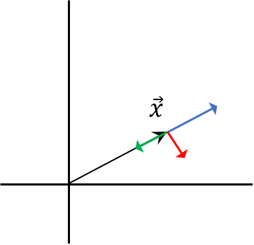
The next more involved type of solution we could look for is a straight-line solution. The idea is that this solution will either move directly (in a straight-line) towards or away from the origin. In the first order autonomous equation case, all of our solutions did this; they either moved towards or away from these equilibrium solutions. This may not be the case for systems, but we can try to find them. If a solution is going to move directly towards or away from the origin, then the direction of change for the solution must be parallel to the position vector. In Figure 4.4.1, the vectors that point in the same or opposite direction of \(\vec{x}\) will give rise to a straight-line solution, but vectors that do not point in this direction will give solutions that do not follow a straight-line through the origin.
We find the eigenvalues \(\lambda_1\text{,}\)\(\lambda_2\text{,}\) …, \(\lambda_n\) of the matrix \(P\text{,}\) and corresponding eigenvectors \(\vec{v}_1\text{,}\)\(\vec{v}_2\text{,}\) …, \(\vec{v}_n\text{.}\) Now we notice that the functions \(\vec{v}_1 e^{\lambda_1 t}\text{,}\)\(\vec{v}_2 e^{\lambda_2 t}\text{,}\) …, \(\vec{v}_n e^{\lambda_n t}\) are solutions of the homogeneous system of equations and hence \(\vec{x} = c_1 \vec{v}_1 e^{\lambda_1 t} +
c_2 \vec{v}_2 e^{\lambda_2 t} + \cdots +
c_n \vec{v}_n e^{\lambda_n t}\) is a solution by superposition.
Take \({\vec{x}}' = P\vec{x}\text{.}\) If \(P\) is an \(n \times n\) constant matrix that has \(n\) distinct real eigenvalues \(\lambda_1\text{,}\)\(\lambda_2\text{,}\) …, \(\lambda_n\text{,}\) then there exist \(n\) linearly independent corresponding eigenvectors \(\vec{v}_1\text{,}\)\(\vec{v}_2\text{,}\) …, \(\vec{v}_n\text{,}\) and the general solution to \({\vec{x}}' = P\vec{x}\) can be written as
Earlier, we found the eigenvalues are \(1,2,3\text{.}\) We found the eigenvector \(\left[ \begin{smallmatrix} 1 \\ 1 \\ 0 \end{smallmatrix} \right]\) for the eigenvalue 3. Similarly we find the eigenvector \(\left[ \begin{smallmatrix} 1 \\ -1 \\ 0 \end{smallmatrix} \right]\) for the eigenvalue 1, and \(\left[ \begin{smallmatrix} 0 \\ 1 \\ -1 \end{smallmatrix} \right]\) for the eigenvalue 2 (exercise: check). Hence our general solution is
Overall, the process for finding the solution for real and distinct eigenvalues is to first find the eigenvalues and eigenvectors of the matrix \(P\text{.}\) Once we have these, we get \(n\) linearly independent solutions of the form \(\vec{x}_i(t) = \vec{v}_ie^{\lambda_i t}\text{,}\) so that the general solution is of the form
Then, if we need to solve for an initial condition, we figure out the coefficients \(c_1\text{,}\)\(c_2\text{,}\) ..., \(c_n\) to satisfy this condition.
Note: If we write a single homogeneous linear constant coefficient \(n^{\text{th}}\) order equation as a first order system (as we did in Section 4.1), then the eigenvalue equation
Since we are in the case of a constant-coefficient linear system, we start by looking for the eigenvalues and eigenvectors of the coefficient matrix \(P\text{.}\) To do this, we compute
The two equations that you get here are redundant, which is \(3v_1 + 4v_2 = 0\text{.}\) One way to satisfy this is \(v_1 = 4\text{,}\)\(v_2 = -3\text{,}\) so that the eigenvector is \(\left[\begin{smallmatrix} 4 \\ -3 \end{smallmatrix} \right]\text{.}\)
so the eigenvector here is \(\left[ \begin{smallmatrix} 1 \\ -1 \end{smallmatrix} \right]\text{.}\) Therefore, the general solution to this differential equation, by superposition, is
These can be solved in any way, including row reduction. We will start by adding the two equations together, which gives \(c_1 = 2\text{,}\) and then the first equation implies that \(c_2 = -7\text{.}\) Therefore, the solution to the initial value problem is
Now that we have these solutions, we want to get an idea for what they look like in the plane. We spent a lot of time in first order equations looking at direction fields, as well as phase lines for autonomous equations. We want to develope the same type of intuition for two-component systems in the plane, because much intuition can be obtained by studying this simple case. Suppose we use coordinates \((x,y)\) for the plane as usual, and suppose \(P = \left[ \begin{smallmatrix} a & b \\ c & d \end{smallmatrix} \right]\) is a \(2 \times 2\) matrix. Consider the system
\begin{equation}
\begin{bmatrix} x \\ y \end{bmatrix} ' =
P \begin{bmatrix} x \\ y \end{bmatrix}
\qquad
\text{or}
\qquad
\begin{bmatrix} x \\ y \end{bmatrix} ' =
\begin{bmatrix} a & b \\ c & d \end{bmatrix}
\begin{bmatrix} x \\ y \end{bmatrix}
.\tag{4.4.1}
\end{equation}
The system is autonomous (compare this section to Section 1.7) and so we can draw a vector field (see the end of Section 4.1). We will be able to visually tell what the vector field looks like and how the solutions behave, once we find the eigenvalues and eigenvectors of the matrix \(P\text{.}\) The goal is to be able to sketch what the different trajectories of the solutions look like for a variety of initial conditions, as well as classify the general type of picture that results depending on the matrix \(P\text{.}\)
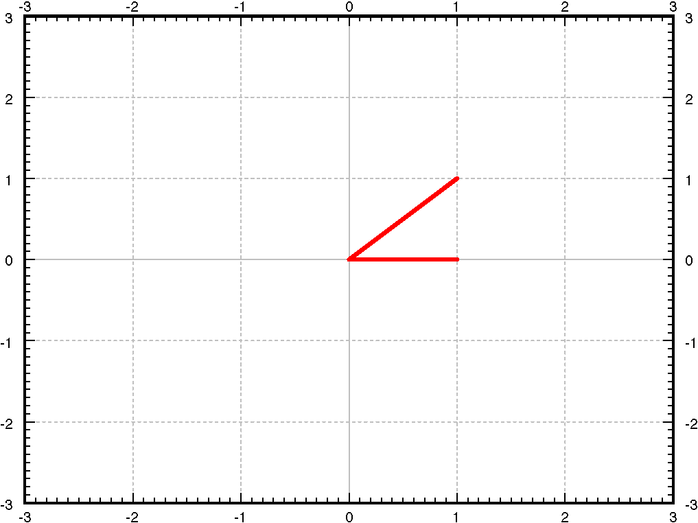
Case 1. Suppose that the eigenvalues of \(P\) are real and positive. We find two corresponding eigenvectors and plot them in the plane. For example, take the matrix \(\left[ \begin{smallmatrix} 1 & 1 \\ 0 & 2 \end{smallmatrix}
\right]\text{.}\) The eigenvalues are 1 and 2 and corresponding eigenvectors are \(\left[ \begin{smallmatrix} 1 \\ 0 \end{smallmatrix} \right]\) and \(\left[ \begin{smallmatrix} 1 \\ 1 \end{smallmatrix} \right]\text{.}\) See Figure 4.4.6.
Suppose the point \((x,y)\) is on the line determined by an eigenvector \(\vec{v}\) for an eigenvalue \(\lambda\text{.}\) That is, \(\left[ \begin{smallmatrix} x \\ y \end{smallmatrix} \right] = \alpha \vec{v}\) for some scalar \(\alpha\text{.}\) Then
\begin{equation*}
\begin{bmatrix} x \\ y \end{bmatrix} '
=
P \begin{bmatrix} x \\ y \end{bmatrix}
=
P ( \alpha \vec{v} ) = \alpha ( P \vec{v} )
= \alpha \lambda \vec{v} .
\end{equation*}
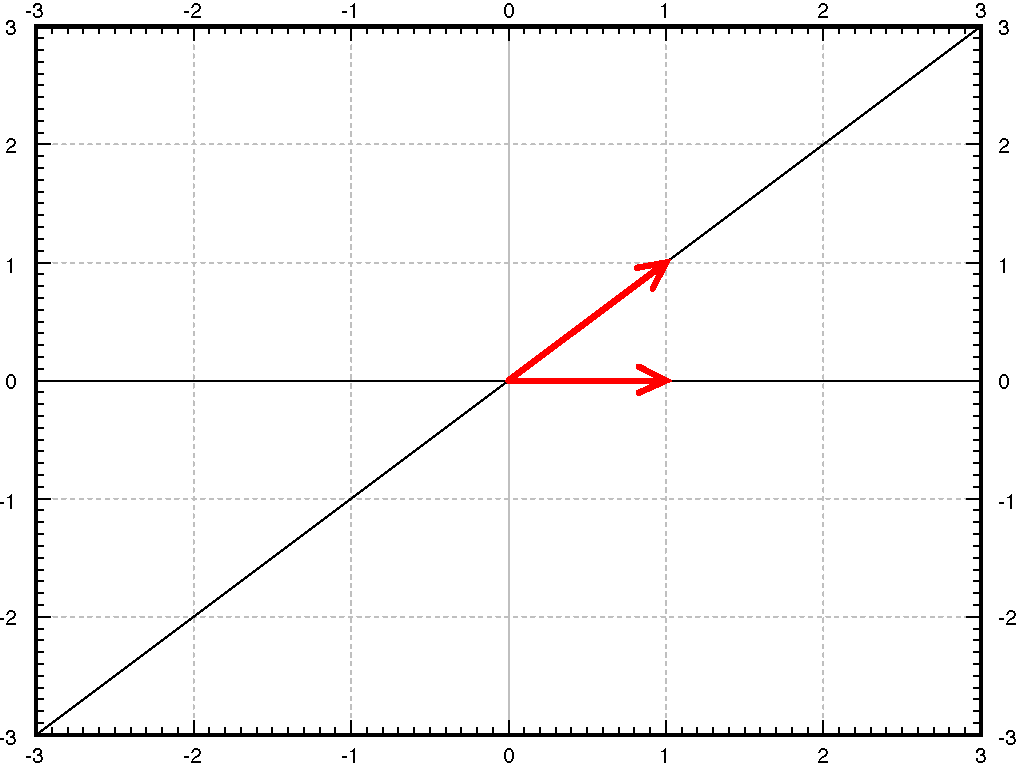
The derivative is a multiple of \(\vec{v}\) and hence points along the line determined by \(\vec{v}\text{.}\) As \(\lambda > 0\text{,}\) the derivative points in the direction of \(\vec{v}\) when \(\alpha\) is positive and in the opposite direction when \(\alpha\) is negative. Let us draw the lines determined by the eigenvectors, and let us draw arrows on the lines to indicate the directions. See Figure 4.4.7.
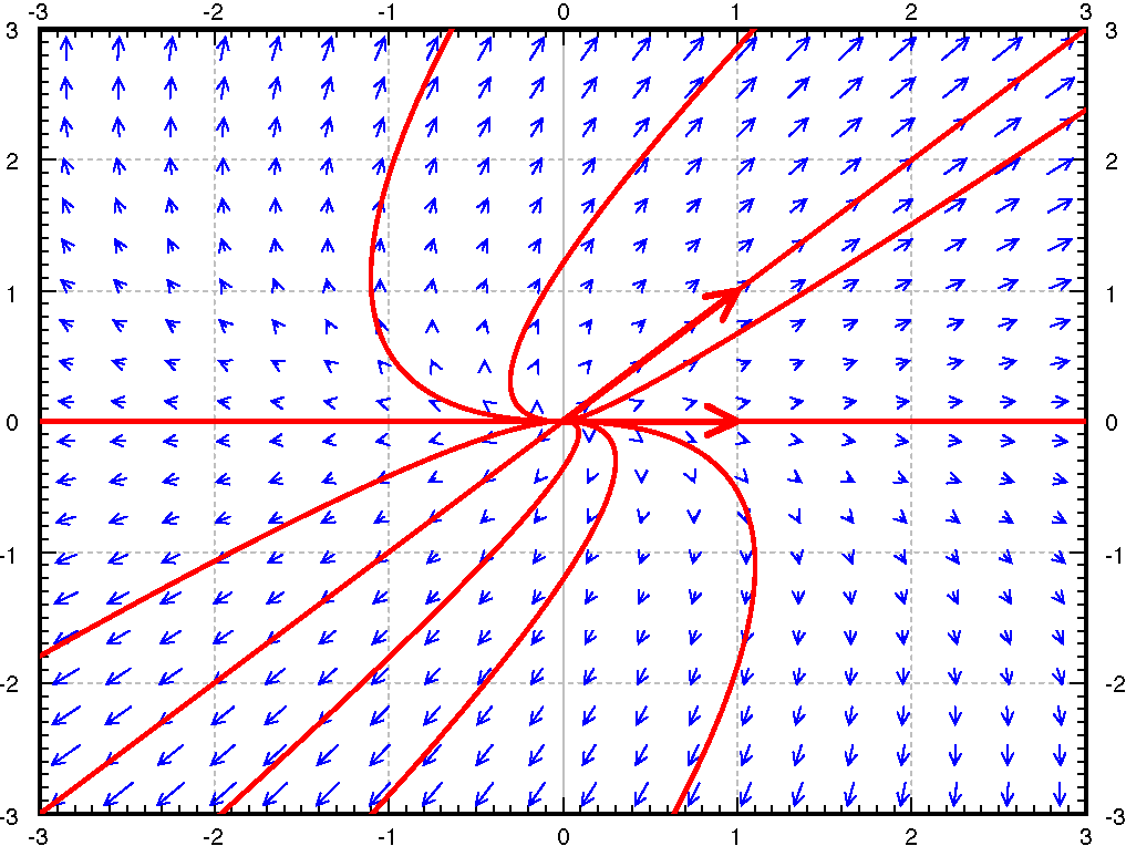
We fill in the rest of the arrows for the vector field and we also draw a few solutions. See Figure 4.4.8. The picture looks like a source with arrows coming out from the origin. Hence we call this type of picture a source or sometimes an unstable node. Notice the two eigenvectors are drawn on the entire vector field figure with arrows, and the straight-line solutions follow them.
We also need to look at how the solution curves are drawn to determine the appropriate shape, even when we don’t have the vector field. In this example, we have two positive eigenvalues, with \(\left[\begin{smallmatrix} 1 \\ 0 \end{smallmatrix}\right]\) as an eigenvector for eigenvalue 1, and \(\left[\begin{smallmatrix} 1 \\ 1 \end{smallmatrix}\right]\) as an eigenvector for eigenvalue 2, which gives rise to a general solution
As \(t\) gets larger, the term with \(e^{2t}\) on it is larger and more important, so the solution curves move parallel to the \(\left[\begin{smallmatrix} 1 \\ 1 \end{smallmatrix}\right]\) line as \(t\rightarrow \infty\text{,}\) which in this case, means as the solution goes away from the origin. In the other direction, as \(t \rightarrow -\infty\text{,}\) the \(e^{2t}\) term vanishes first, meaning the \(e^t\) term is more important. So the solution curves will leave from the origin (since this happens as \(t \rightarrow -\infty\)) in the direction of the \(\left[\begin{smallmatrix} 1 \\ 0 \end{smallmatrix}\right]\) line.
That is exactly what we see in Figure 4.4.8; the solutions leave the origin along the \(\left[\begin{smallmatrix} 1 \\ 0 \end{smallmatrix}\right]\) line and then head to infinity parallel to the \(\left[\begin{smallmatrix} 1 \\ 1 \end{smallmatrix}\right]\) line. Within the figure here, they don’t quite get parallel to those lines, but they will get more and more parallel as they get farther away from the origin.
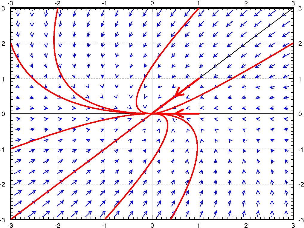
Case 2. Suppose both eigenvalues are negative. For example, take the negation of the matrix in case 1, \(\left[ \begin{smallmatrix} -1 & -1 \\ 0 & -2 \end{smallmatrix} \right]\text{.}\) The eigenvalues are \(-1\) and \(-2\) and corresponding eigenvectors are the same, \(\left[ \begin{smallmatrix} 1 \\ 0 \end{smallmatrix} \right]\) and \(\left[ \begin{smallmatrix} 1 \\ 1 \end{smallmatrix} \right]\text{.}\) The calculation and the picture are almost the same. The only difference is that the eigenvalues are negative and hence all arrows are reversed. We get the picture in Figure 4.4.9. We call this kind of picture a sink or an asymptotically stable node.
In terms of the shape of the solution curves, the same type of argument works. This general solution will have terms involving \(e^{-t}\) and \(e^{-2t}\text{.}\) The solution is tending towards the origin as \(t \rightarrow \infty\text{,}\) and as it does, the \(e^{-2t}\) term vanishes first. Therefore, the solution goes to the origin along the line corresponding to \(e^{-t}\text{,}\) which is \(\left[\begin{smallmatrix} 1 \\ 0 \end{smallmatrix}\right]\text{.}\) As \(t \rightarrow -\infty\text{,}\) the reverse happens, and the \(e^{-2t}\) term matters more, so the solution comes in from infinity parallel to the \(\left[\begin{smallmatrix} 1 \\ 1 \end{smallmatrix}\right]\) line. Exactly where this “parallel” component of the line is depends on the initial condition. This is again what we see in Figure 4.4.9.
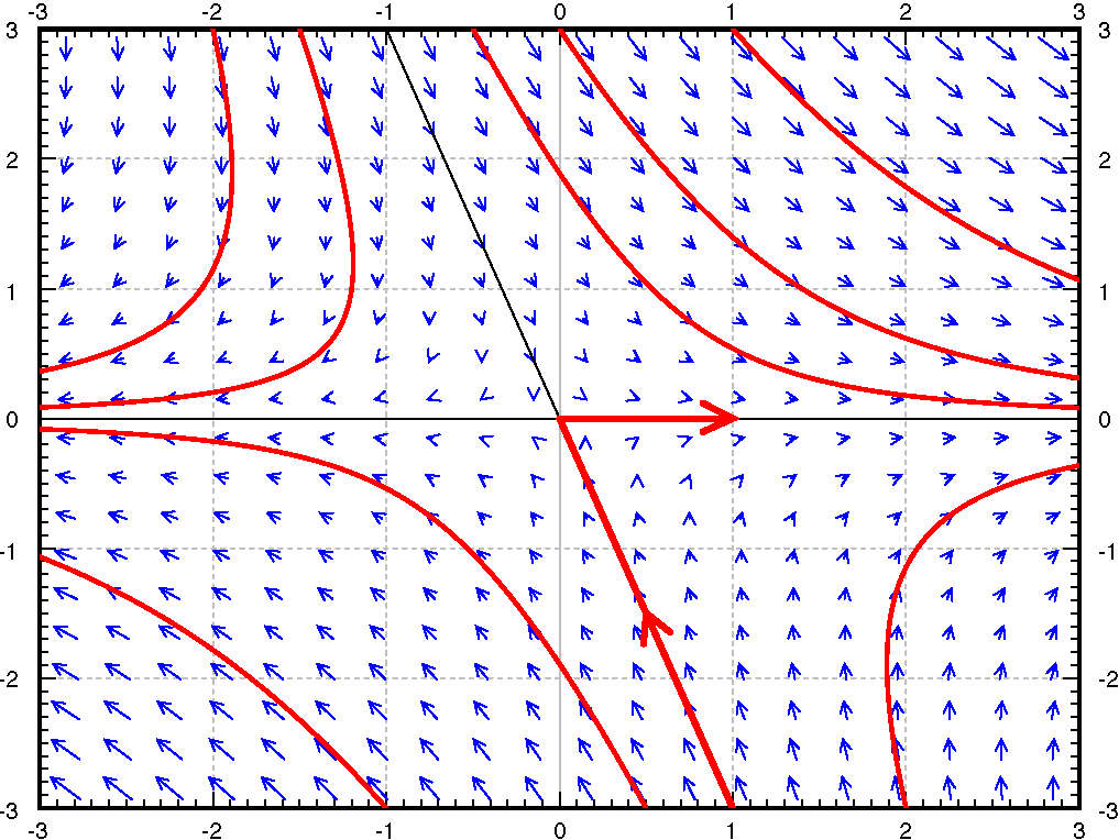
Case 3. Suppose one eigenvalue is positive and one is negative. For example the matrix \(\left[ \begin{smallmatrix} 1 & 1 \\ 0 & -2 \end{smallmatrix} \right]\text{.}\) The eigenvalues are \(1\) and \(-2\) and corresponding eigenvectors are \(\left[ \begin{smallmatrix} 1 \\ 0 \end{smallmatrix} \right]\) and \(\left[ \begin{smallmatrix} 1 \\ -3 \end{smallmatrix} \right]\text{.}\) We reverse the arrows on one line (corresponding to the negative eigenvalue) and we obtain the picture in Figure 4.4.10. We call this picture a saddle point.
As \(t\rightarrow \infty\text{,}\) the \(e^{-2t}\) term vanishes, so only the \(\left[\begin{smallmatrix} 1 \\ 0 \end{smallmatrix}\right]e^t\) term remains, meanin the solution approaches the \(\left[\begin{smallmatrix} 1 \\ 0 \end{smallmatrix}\right]\) line. In the other direction, as \(t \rightarrow -\infty\text{,}\) the \(e^t\) term vanishes, meaning that our solution approaches the straight-line solution with negative eigenvalue, which in this case is the \(\left[\begin{smallmatrix} 1 \\ -3 \end{smallmatrix}\right]\) line.
Find the general solution of \(x_1' = 2 x_1\text{,}\)\(x_2' = 3 x_2\) using the eigenvalue method (first write the system in the form \({\vec{x}}' = A \vec{x}\)).
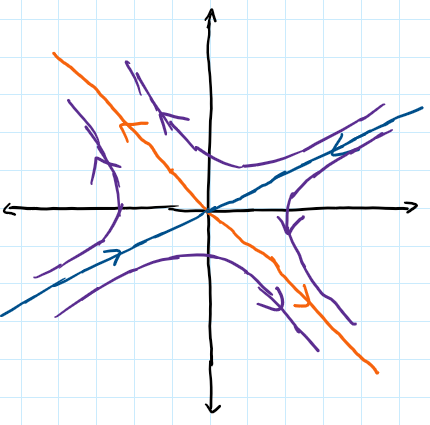
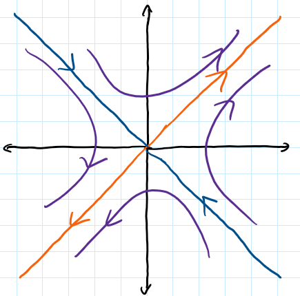
Find the general solution of \(x_1' = 3 x_1 + x_2\text{,}\)\(x_2' = 2 x_1 + 4 x_2\) using the eigenvalue method and sketch the phase portrait for this system of differential equations.
Amino acid dating can be used by forensic scientists to determine the time of death in situations where other techniques might not work. These amino acids are sneaky, and they exist in a left-handed form (L) and a right-handed form (D), which are called enantiomers. While you’re alive, your body keeps all your amino acids in the L form. Once you die, your body no longer regulates your amino acids, and every so often they flip a coin and decide whether to switch into the opposite form. This way, when someone finds your body in a dumpster, they can pull out your teeth and measure the racemization ratio, which is the ratio of D-enantiomers to L-enantiomers.
Denote by \(D(t)\) and \(L(t)\text{,}\) respectively, the proportions of D- and L-enantiomers found in your teeth, where \(t\) is measured in years after death. Since this is Math class, the proportions are governed by a system of differential equations, such as
\begin{equation}
\begin{bmatrix} L' \\ D' \end{bmatrix} = \begin{bmatrix} -.02& .02\\ .02 & -.02 \end{bmatrix}\begin{bmatrix} L\\ D \end{bmatrix}.\tag{4.4.2}
\end{equation}
Solve (4.4.2) with initial conditions \(D(0) = 0\) and \(L(0) = 1\text{,}\) and express the solution in component form. Describe what happens to the quantities \(D(t)\) and \(L(t)\) in the long run.
Let \(a,b,c,d,e,f\) be numbers. Find the eigenvalues of \(\left[ \begin{smallmatrix}
a & b & c \\
0 & d & e \\
0 & 0 & f \\
\end{smallmatrix} \right]\text{.}\)