Except for a few brief detours in Chapter 1, we considered mostly linear equations. Linear equations suffice in many applications, but in reality most phenomena require nonlinear equations. Nonlinear equations, however, are notoriously more difficult to understand than linear ones, and many strange new phenomena appear when we allow our equations to be nonlinear.
Not to worry, we did not waste all this time studying linear equations. Nonlinear equations can often be approximated by linear ones if we only need a solution “locally”, for example, only for a short period of time, or only for certain parameters. Understanding specific linear equations can also give us qualitative understanding about a more general nonlinear problem. The idea is similar to what you did in calculus in trying to approximate a function by a line with the right slope.
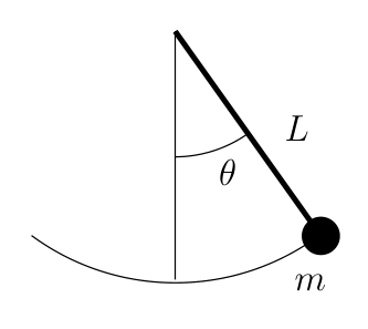
In Section 2.4 we looked at the pendulum of length \(L\text{.}\) The goal was to solve for the angle \(\theta(t)\) as a function of the time \(t\text{.}\) The equation for the setup is the nonlinear equation
While the solution to the linear equation is not exactly what we were looking for, it is rather close to the original, as long as the angle \(\theta\) is small and the time period involved is short.
You might ask: Why don’t we just solve the nonlinear problem? Well, it might be very difficult, impractical, or impossible to solve analytically, depending on the equation in question. We may not even be interested in the actual solution, we might only be interested in some qualitative idea of what the solution is doing. For example, what happens as time goes to infinity?
where \(f(x,y)\) and \(g(x,y)\) are functions of two variables, and the derivatives are taken with respect to time \(t\text{.}\) Solutions are functions \(x(t)\) and \(y(t)\) such that
The way we will analyze the system is very similar to Section 1.7, where we studied a single autonomous equation. The ideas in two dimensions are the same, but the behavior can be far more complicated.
It may be best to think of the system of equations as the single vector equation
\begin{equation}
\begin{bmatrix} x \\ y \end{bmatrix} ' =
\begin{bmatrix} f(x,y) \\ g(x,y) \end{bmatrix} .\tag{5.1.1}
\end{equation}
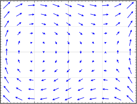
As in Section 4.1 we draw the phase portrait (or phase diagram), where each point \((x,y)\) corresponds to a specific state of the system. We draw the vector field given at each point \((x,y)\) by the vector \(\left[ \begin{smallmatrix} f(x,y) \\ g(x,y) \end{smallmatrix} \right]\text{.}\) And as before if we find solutions, we draw the trajectories by plotting all points \(\bigl(x(t),y(t)\bigr)\) for a certain range of \(t\text{.}\)
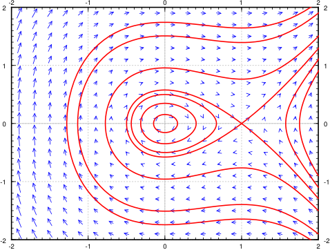
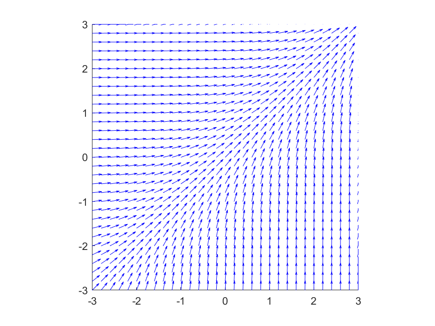
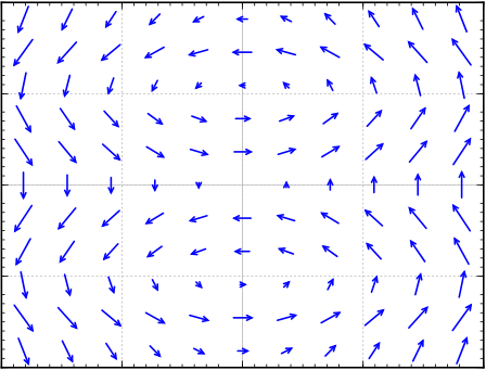
From the phase portrait it should be clear that even this simple system has fairly complicated behavior. Some trajectories keep oscillating around the origin, and some go off towards infinity. We will return to this example often, and analyze it completely in this (and the next) section.
If we zoom into the diagram near a point where \(\left[ \begin{smallmatrix} f(x,y) \\ g(x,y) \end{smallmatrix} \right]\) is not zero, then nearby the arrows point generally in essentially that same direction and have essentially the same magnitude. In other words the behavior is not that interesting near such a point. We are of course assuming that \(f(x,y)\) and \(g(x,y)\) are continuous.
Let us concentrate on those points in the phase diagram above where the trajectories seem to start, end, or go around. We see two such points: \((0,0)\) and \((1,0)\text{.}\) The trajectories seem to go around the point \((0,0)\text{,}\) and they seem to either go in or out of the point \((1,0)\text{.}\) These points are precisely those points where the derivatives of both \(x\) and \(y\) are zero.
The critical points are where the behavior of the system is in some sense the most complicated. If \(\left[ \begin{smallmatrix} f(x,y) \\ g(x,y) \end{smallmatrix} \right]\) is zero, then nearby, the vector can point in any direction whatsoever. Also, the trajectories are either going towards, away from, or around these points, so if we are looking for long-term qualitative behavior of the system, we should look at what is happening near the critical points.
Critical points are also sometimes called equilibria, since we have so-called equilibrium solutions at critical points. If \((x_0,y_0)\) is a critical point, then we have the solutions
The discussion here should seem a bit familiar; it is the same as how we formulated equilibrium solutions to autonomous differential equations in Section 1.7.
where \(A\) is an invertible matrix, the only critical point is the origin \((0,0)\text{.}\) Since \(A\) is invertible, the only vector that satisfies \(A\vec{x} = 0\) is \(\vec{x} = 0\text{,}\) see Section 3.4. (This also applies beyond two variables, but we’ll stick to that for simplicity.) In Section 4.7 we studied the behavior of a homogeneous linear system of two equations near a critical point. Let us put the understanding we gained in that section to good use understanding what happens near critical points of nonlinear systems.
In calculus we learned to estimate a function by taking its derivative and linearizing. We work similarly with nonlinear systems of ODE. Suppose \((x_0,y_0)\) is a critical point. In order to linearize the system of differential equations, we want to linearize the two functions \(f(x,y)\) and \(g(x,y)\) that define this system. To do so, we will replace \(f\) and \(g\) by the tangent plane approximation to the functions. That is, if we set \(z = f(x,y)\text{,}\) the tangent plane is given by
The idea of linearization in calculus was that we could use the tangent line or tangent plane to approximate a function near to a given point. For systems of differential equations, the idea is that we can approximate the solutions to the system of differential equations by the solutions to the linearized systems as long as we stay near the critical point. That means that we can approximate the solution to
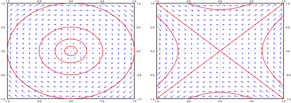
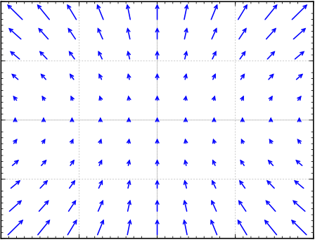
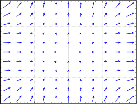
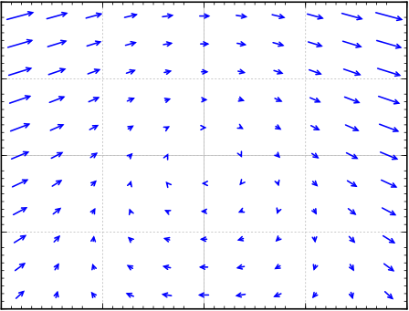
The phase diagrams of the two linearizations at the point \((0,0)\) and \((1,0)\) are given in Figure 5.1.7. Note that the variables are now \(u\) and \(v\text{.}\) Compare with Figure 5.1.3, and look especially at the behavior near the critical points.
Figure5.1.7.Phase diagram with some trajectories of linearizations at the critical points \((0,0)\)$ (left) and \((1,0)\) (right) of \(x' = y\text{,}\)\(y' = -x+x^2\text{.}\)
SubsectionIsolated critical points and almost linear systems
The next step in this process is to try to figure out a way to analyze what is happening to a non-linear system of differential equations near equilibrium solutions without using a slope field/phase portrait. We would like to be able to determine this from the equations alone, not any of the pictures that come from them. Thankfully, our ability to analyze linear systems helps us accomplish this goal.
That is, if we zoom in far enough it is the only critical point we see. In the example above, the critical point was isolated. If on the other hand there would be a whole curve of critical points, then it would not be isolated. For example, the system
A system is called almost linear at a critical point \((x_0,y_0)\text{,}\) if the critical point is isolated and the Jacobian matrix at the point is invertible, or equivalently if the linearized system has an isolated critical point.
This is also equivalent to zero not being an eigenvalue of the Jacobian matrix at the critical point. In such a case, the nonlinear terms are very small and the system behaves like its linearization, at least if we are close to the critical point.
For example, the system in Example 5.1.2 and Example 5.1.6 has two isolated critical points \((0,0)\) and \((0,1)\text{,}\) and is almost linear at both critical points as the Jacobian matrices at both points, \(\left[ \begin{smallmatrix} 0 & 1 \\ -1 & 0 \end{smallmatrix} \right]\) and \(\left[ \begin{smallmatrix} 0 & 1 \\ 1 & 0 \end{smallmatrix} \right]\text{,}\) are invertible.
is zero when \((x,y) = (0,0)\text{.}\) So the system is not almost linear. Even a worse example is the system \(x' = x\text{,}\)\(y' = x^2\text{,}\) which does not have isolated critical points; \(x'\) and \(y'\) are both zero whenever \(x=0\text{,}\) that is, the entire \(y\)-axis.
Fortunately, most often critical points are isolated, and the system is almost linear at the critical points. So if we learn what happens there, we will have figured out the majority of situations that arise in applications.
SubsectionStability and classification of isolated critical points
Once we have an isolated critical point, the system is almost linear at that critical point, and we computed the associated linearized system, we can classify what happens to the solutions. The classifications for linear two-variable systems from Section 4.7 are generally the same as what we use here, with one minor caveat. Let us list the behaviors depending on the eigenvalues of the Jacobian matrix at the critical point in Table 5.1.10. This table is very similar to Table 4.7.1, with the exception of missing “center” points. The repeated eigenvalue cases are also missing. They behave similarly to the real eigenvalue descriptions in the table below, but similar to centers, the behavior can change slightly. It can behave like either a spiral or a node, but will be either a source or sink based on the sign of the repeated eigenvalue. We will discuss centers later, as they are more complicated.
Let \((x_0, y_0)\) be a critical point for a non-linear system of two differential equations.
We say that the critical point is a stable critical point if, given any small distance \(\epsilon\) to \((x_0,y_0)\text{,}\) and any initial condition within a perhaps smaller radius around \((x_0,y_0)\text{,}\) the trajectory of the system never goes further away from \((x_0,y_0)\) than \(\epsilon\text{.}\)
The critical point is an unstable critical point if it is not stable; that is, there are trajectories that start within a distance \(\epsilon\) of \((x_0, y_0)\) and end up farther than \(\epsilon\) from that point.
The critical point is called asymptotically stable if given any initial condition sufficiently close to \((x_0,y_0)\) and any solution \(\bigl( x(t), y(t) \bigr)\) satisfying that condition, then
Informally, a point is stable if we start close to a critical point and follow a trajectory we either go towards, or at least not away from, this critical point. If the point is asymptotically stable, then any trajectory for a sufficiently close initial condition goes towards the critical point \((x_0,y_0)\text{,}\) and unstable means that, in general, trajectories move away from the critical point.
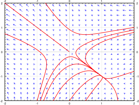
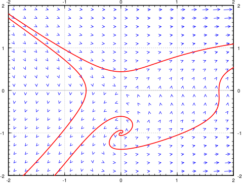
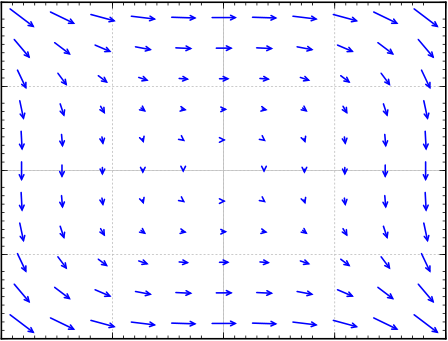
See Figure 5.1.13 for the phase diagram. Let us find the critical points. These are the points where \(-y-x^2 = 0\) and \(-x+y^2=0\text{.}\) The first equation means \(y = -x^2\text{,}\) and so \(y^2 = x^4\text{.}\) Plugging into the second equation we obtain \(-x+x^4 = 0\text{.}\) Factoring we obtain \(x(1-x^3)=0\text{.}\) Since we are looking only for real solutions we get either \(x=0\) or \(x=1\text{.}\) Solving for the corresponding \(y\) using \(y = -x^2\text{,}\) we get two critical points, one being \((0,0)\) and the other being \((1,-1)\text{.}\) Clearly the critical points are isolated.
At the point \((0,0)\) we get the matrix \(\left[ \begin{smallmatrix} 0 & -1 \\ -1 & 0 \end{smallmatrix} \right]\) and so the two eigenvalues are \(1\) and \(-1\text{.}\) As the matrix is invertible, the system is almost linear at \((0,0)\text{.}\) As the eigenvalues are real and of opposite signs, we get a saddle point, which is an unstable equilibrium point. Looking at the phase portrait, we can see trajectories that would start near \((0,0)\) and end up farther away from \((0,0)\text{.}\) These trajectories may end up at \((1,-1)\text{,}\) but that is away from \((0,0)\text{.}\)
At the point \((1,-1)\) we get the matrix \(\left[ \begin{smallmatrix} -2 & -1 \\ -1 & -2 \end{smallmatrix} \right]\) and computing the eigenvalues we get \(-1\text{,}\)\(-3\text{.}\) The matrix is invertible, and so the system is almost linear at \((1,-1)\text{.}\) As we have real eigenvalues and both negative, the critical point is a sink, and therefore an asymptotically stable equilibrium point. That is, if we start with any point \((x(0),y(0))\) close to \((1,-1)\) as an initial condition and plot a trajectory, it approaches \((1,-1)\text{.}\) In other words,
As you can see from the diagram, this behavior is true even for some initial points quite far from \((1,-1)\text{,}\) but it is definitely not true for all initial points.
First let us find the critical points. These are the points where \(y+y^2e^x = 0\) and \(x=0\text{.}\) Simplifying we get \(0=y+y^2 = y(y+1)\text{.}\) So the critical points are \((0,0)\) and \((0,-1)\text{,}\) and hence are isolated. Let us compute the Jacobian matrix:
At the point \((0,0)\) we get the matrix \(\left[ \begin{smallmatrix} 0 & 1 \\ 1 & 0 \end{smallmatrix} \right]\) and so the two eigenvalues are \(1\) and \(-1\text{.}\) As the matrix is invertible, the system is almost linear at \((0,0)\text{.}\) And, as the eigenvalues are real and of opposite signs, we get a saddle point, which is an unstable equilibrium point.
At the point \((0,-1)\) we get the matrix \(\left[ \begin{smallmatrix} 1 & -1 \\ 1 & 0 \end{smallmatrix} \right]\) whose eigenvalues are \(\frac{1}{2} \pm i \frac{\sqrt{3}}{2}\text{.}\) The matrix is invertible, and so the system is almost linear at \((0,-1)\text{.}\) As we have complex eigenvalues with positive real part, the critical point is a spiral source, and therefore an unstable equilibrium point.
Recall, a linear system with a center means that trajectories travel in closed elliptical orbits in some direction around the critical point. Such a critical point we call a center or a stable center. It is not an asymptotically stable critical point, as the trajectories never approach the critical point, but at least if you start sufficiently close to the critical point, you stay close to the critical point. The simplest example of such behavior is the linear system with a center. Another example is the critical point \((0,0)\) in Example 5.1.2.
The trouble with a center in a nonlinear system is that whether the trajectory goes towards or away from the critical point is governed by the sign of the real part of the eigenvalues of the Jacobian matrix, and the Jacobian matrix in a nonlinear system changes from point to point. Since this real part is zero at the critical point itself, it can have either sign nearby, meaning the trajectory could be pulled towards or away from the critical point.
At \((0,0)\) the Jacobian matrix is \(\left[ \begin{smallmatrix}
0 & 1 \\
-1 & 0 \\
\end{smallmatrix} \right]\text{,}\) which has eigenvalues \(\pm i\text{.}\) So the linearization has a center.
Using the quadratic equation, the eigenvalues of the Jacobian matrix at any point \((x,y)\) are
\begin{equation*}
\lambda =
\frac{3}{2}y^2 \pm
i
\frac{\sqrt{4-9y^4}}{2} .
\end{equation*}
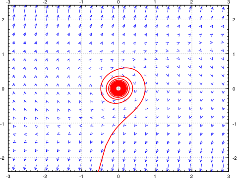
At any point where \(y \not= 0\) (so at most points near the origin), the eigenvalues have a positive real part (\(y^2\) can never be negative). This positive real part pulls the trajectory away from the origin. A sample trajectory for an initial condition near the origin is given in Figure 5.1.17.
The same process could be carried out with the system \(x'=y, y' = -x-y^3\text{.}\) This one will also have a center as the linearization at the origin, but the non-linear system will have a spiral sink at the origin. The moral of the example is that further analysis is needed when the linearization has a center. The analysis will in general be more complicated than in the example above, and is more likely to involve case-by-case consideration. Such a complication should not be surprising to you. By now in your mathematical career, you have seen many places where a simple test is inconclusive, recall for example the second derivative test for maxima or minima, and requires more careful, and perhaps ad hoc analysis of the situation.
\(x'=ax+by+f(x,y)\text{,}\)\(y'=cx+dy+g(x,y)\text{,}\) where \(f(0,0) = 0\text{,}\)\(g(0,0) = 0\text{,}\) and all first partial derivatives of \(f\) and \(g\) are also zero at \((0,0)\text{,}\) that is, \(\frac{\partial f}{\partial x}(0,0) =
\frac{\partial f}{\partial y}(0,0) =
\frac{\partial g}{\partial x}(0,0) =
\frac{\partial g}{\partial y}(0,0) = 0\text{.}\)
For each of the critical points, determine the behavior and classify the type of solution that the linearized system will have around that critical point.
For each of the critical points, determine the behavior and classify the type of solution that the linearized system will have around that critical point.
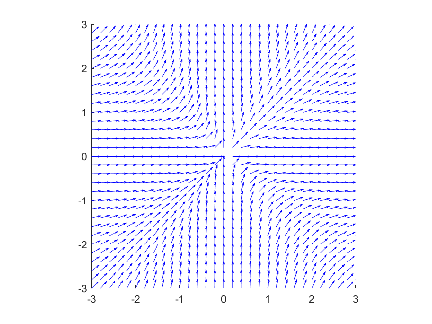
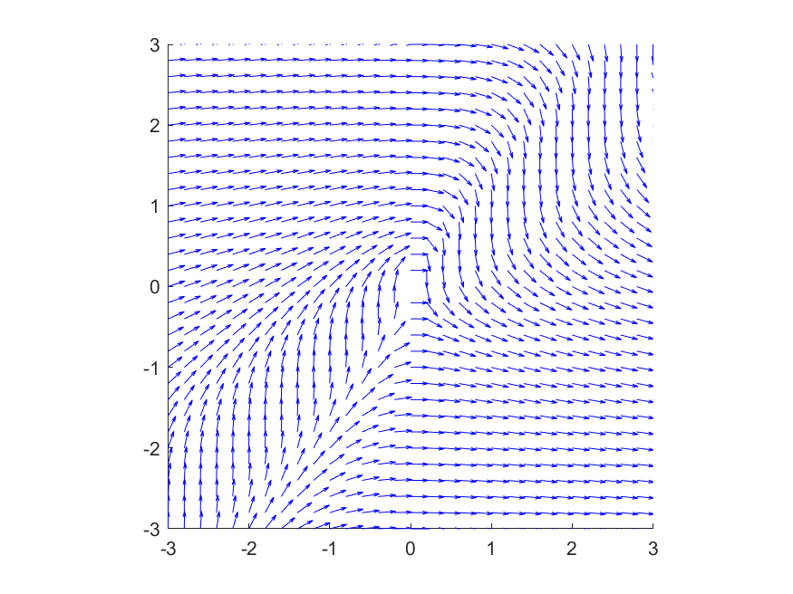
The idea of critical points and linearization works in higher dimensions as well. You simply make the Jacobian matrix bigger by adding more functions and more variables. For the following system of 3 equations find the critical points and their linearizations:
Critical points are \((0,0,0)\text{,}\) and \((-1, 1, -1)\text{.}\) The linearization at the origin using variables \(u=x\text{,}\)\(v=y\text{,}\)\(w=z\) is \(u' = u\text{,}\)\(v'=-v\text{,}\)\(z' = w\text{.}\) The linearization at the point \((-1,1,-1)\) using variables \(u=x+1\text{,}\)\(v=y-1\text{,}\)\(w=z+1\) is \(u'=u-2w\text{,}\)\(v'=-v-2w\text{,}\)\(w'=w-2u\text{.}\)
Any two-dimensional non-autonomous system \(x'=f(x,y,t)\text{,}\)\(y'=g(x,y,t)\) can be written as a three-dimensional autonomous system (three equations). Write down this autonomous system using the variables \(u\text{,}\)\(v\text{,}\)\(w\text{.}\)
In the example \(x'=y\text{,}\)\(y'=y^3-x\) show that for any trajectory, the distance from the origin is an increasing function. Conclude that the origin behaves like is a spiral source. Hint: Consider \(f(t) =
{\bigl(x(t)\bigr)}^2 +
{\bigl(y(t)\bigr)}^2\) and show it has positive derivative.
Find and analyze all critical points of the system \(x' = y\text{,}\)\(y' = -x - y^3\text{.}\) Use the ideas from Exercise 19 to show that the solutions to this problem move towards the origin as \(t\) grows.
Derive an analogous classification of critical points for equations in one dimension, such as \(x'= f(x)\) based on the derivative. A point \(x_0\) is critical when \(f(x_0) = 0\) and almost linear if in addition \(f'(x_0) \not= 0\text{.}\) Figure out if the critical point is stable or unstable depending on the sign of \(f'(x_0)\text{.}\) Explain. Hint: see Section 1.7.