Forced oscillations and resonance

Section 2.6 Forced oscillations and resonance

Objectives

After this section, you will be able to:

Write differential equations to model forced oscillators (like masses on springs),
🔗

🔗
Identify when beats, pure resonance, and practical resonance can occur, and
🔗

🔗
Use proper terminology around transient and steady periodic solutions when discussing these problems.
🔗

🔗

ALT TEXT HERE — Figure 2.6.1. Schematic of the mass-spring system with an applied force.
🔗

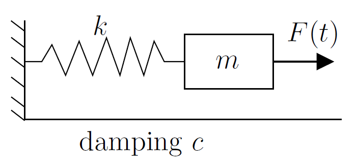
Let us return back to the example of a mass on a spring. We examine the case of forced oscillations, which we did not yet handle. That is, we consider the equation

\begin{equation*} mx'' + \gamma x' + kx = F(t) , \end{equation*}

for some nonzero $F(t)\text{.}$ The setup is again: $m$ is mass, $\gamma$ is friction, $k$ is the spring constant, and $F(t)$ is an external force acting on the mass.

🔗

We are interested in periodic forcing, such as noncentered rotating parts, or perhaps loud sounds, or other sources of periodic force.

🔗

Subsection Undamped forced motion and resonance

First let us consider undamped ($\gamma =0$) motion. We have the equation

\begin{equation*} mx'' + kx = F_0 \cos (\omega t) . \end{equation*}

This equation has the complementary solution (solution to the associated homogeneous equation)

\begin{equation*} x_c = C_1 \cos (\omega_0 t) + C_2 \sin (\omega_0 t) , \end{equation*}

where $\omega_0 = \sqrt{\nicefrac{k}{m}}$ is the natural frequency (angular). It is the frequency at which the system “wants to oscillate” without external interference.

🔗

Suppose that $\omega_0 \not= \omega\text{.}$ We try the solution $x_p = A \cos (\omega t)$ and solve for $A\text{.}$ We do not need a sine in our trial solution as after plugging in we only have cosines. If you include a sine, it is fine; you will find that its coefficient is zero (I could not find a second rhyme).

🔗

We solve using the method of undetermined coefficients. We find that

\begin{equation*} x_p = \frac{F_0}{m(\omega_0^2 - \omega^2)} \cos (\omega t) . \end{equation*}

We leave it as an exercise to do the algebra required.

🔗

The general solution is

\begin{equation*} \mybxbg{ ~~ x = C_1 \cos (\omega_0 t) + C_2 \sin (\omega_0 t) + \frac{F_0}{m(\omega_0^2 - \omega^2)} \cos (\omega t) . ~~ } \end{equation*}

Written another way

\begin{equation*} x = C \cos (\omega_0 t - \gamma) + \frac{F_0}{m(\omega_0^2 - \omega^2)} \cos (\omega t) . \end{equation*}

The solution is a superposition of two cosine waves at different frequencies.

🔗

Example 2.6.2.

Take

\begin{equation*} 0.5 x'' + 8 x = 10 \cos (\pi t), \qquad x(0)=0, \qquad x'(0)=0 . \end{equation*}

🔗

Solution.

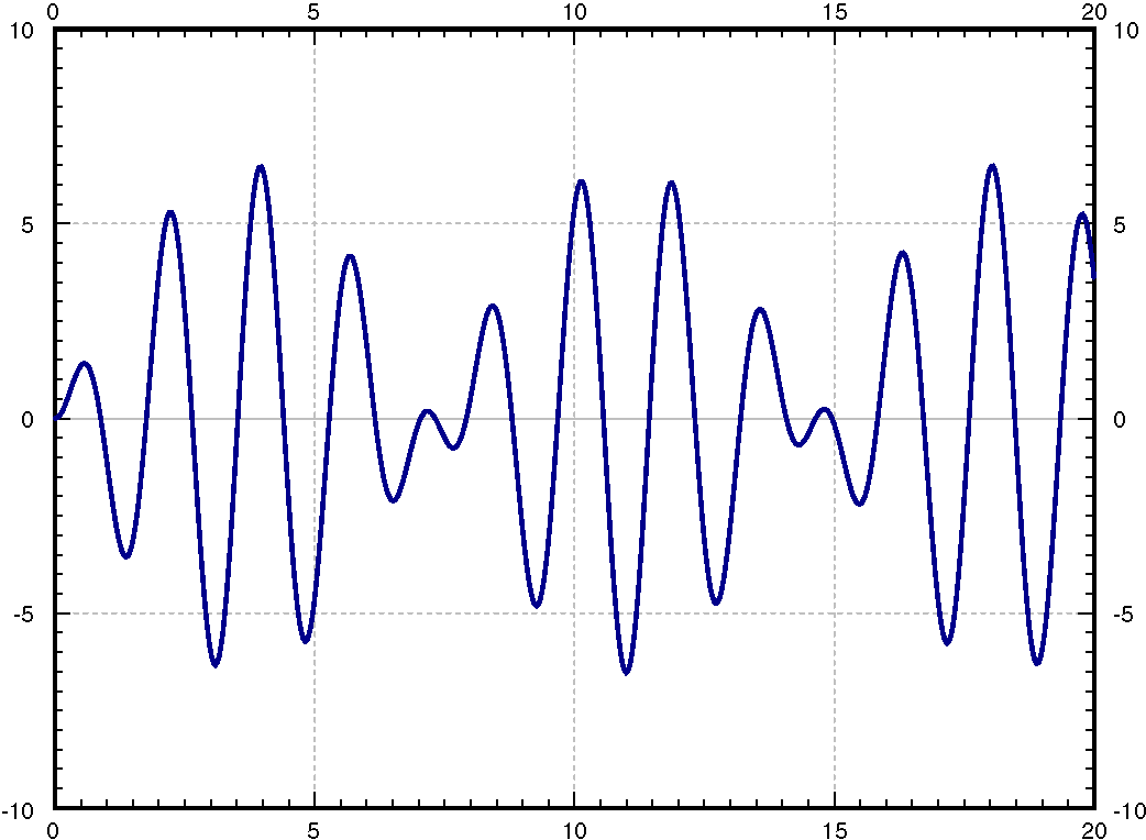
Let us compute. First we read off the parameters: $\omega = \pi\text{,}$ $\omega_0 = \sqrt{\nicefrac{8}{0.5}} = 4\text{,}$ $F_0 = 10\text{,}$ $m=0.5\text{.}$ The general solution is

\begin{equation*} x = C_1 \cos (4 t) + C_2 \sin (4 t) + \frac{20}{16 - \pi^2} \cos (\pi t) . \end{equation*}

🔗

Solve for $C_1$ and $C_2$ using the initial conditions: $C_1 = \frac{-20}{16 - \pi^2}$ and $C_2 = 0\text{.}$ Hence

\begin{equation*} x = \frac{20}{16 - \pi^2} \bigl( \cos (\pi t)- \cos (4 t) \bigr) . \end{equation*}

🔗

Notice the beating behavior in Figure 2.6.3. First use the trigonometric identity

\begin{equation*} 2\sin \left( \frac{A-B}{2} \right) \sin \left( \frac{A+B}{2} \right) = \cos B -\cos A \end{equation*}

to get

\begin{equation*} x = \frac{20}{16 - \pi^2} \left( 2 \sin \left(\frac{4-\pi}{2} t \right) \sin \left( \frac{4+\pi}{2} t \right) \right) . \end{equation*}

The function $x$ is a high frequency wave modulated by a low frequency wave.

🔗

The beating behavior can be experienced even more readily by considering a higher frequency and viewing the resulting function as a sound wave. A sound wave of frequency 440 Hz produces and A4 sound, which is the A above middle C on a piano. This means that the function

\begin{equation*} x_p(t) = \sin(2\pi\cdot 440 t) \end{equation*}

will produce a sound wave equivalent to this A4 sound. In MATLAB, this can be done with the code

🔗

Listing 2.6.4. Playing Sounds in Matlab

🔗

omega0 = 440*2*pi; tVals = linspace(0, 5, 5*8192);
testSound = sin(omega0*tVals);
 sound(testSound);

which will play this pitch for 5 seconds. Now, we want to see what happens if we take a mass-on-a-spring with this natural frequency and apply a forcing function with frequency close to this value. The following code assumes a forcing function of frequency 444 Hz. The multiple of $\omega_0$ in front of the forcing function is only for scaling purposes; otherwise the resulting sound would be too quiet.

🔗

Listing 2.6.5. Plotting Beats in Matlab

🔗

omega = 444*2*pi;
syms ys(t); 
[V] = odeToVectorField(diff(ys, 2) + omega0^2*ys == omega0*cos(omega*t)); 
MS = matlabFunction(V, 'vars', 't', 'Y'); soln = ode45(MS, [0,10], [0,0]);
ySound = deval(soln, tVals); 
ySound = ySound(1, :); 
sound(ySound);

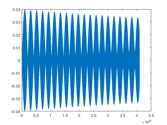
A graph of the solution ySound can be found in Figure 2.6.6. This exhibits the beating behavior before on a large scale. The sound played during this code also shows the beating or amplitude modulation that can happen in these sorts of solutions. In terms of tuning instruments, these beats are some of the main things musicians will listen for to know if their instrument is close to the right pitch, but just slightly off.

🔗

Now suppose $\omega_0 = \omega\text{.}$ We cannot try the solution $A \cos (\omega t)$ and then use the method of undetermined coefficients, since we notice that $\cos (\omega t)$ solves the associated homogeneous equation. Therefore, we try $x_p = A t \cos (\omega t) + B t \sin (\omega t)\text{.}$ This time we need the sine term, since the second derivative of $t \cos (\omega t)$ contains sines. We write the equation

\begin{equation*} x'' + \omega^2 x = \frac{F_0}{m} \cos ( \omega t) . \end{equation*}

Plugging $x_p$ into the left-hand side we get

\begin{equation*} 2 B \omega \cos (\omega t) - 2 A \omega \sin (\omega t) = \frac{F_0}{m} \cos (\omega t) . \end{equation*}

Hence $A = 0$ and $B = \frac{F_0}{2m\omega}\text{.}$ Our particular solution is $\frac{F_0}{2m\omega} \, t \sin (\omega t)$ and our general solution is

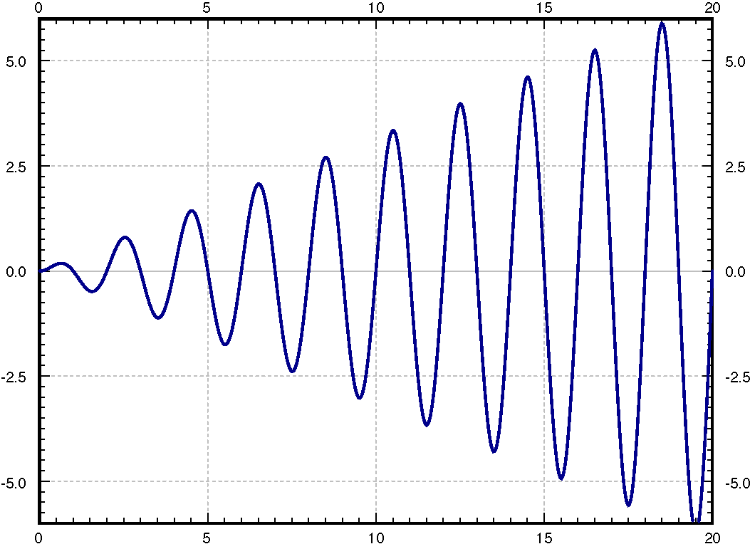
\begin{equation*} x = C_1 \cos (\omega t) + C_2 \sin (\omega t) + \frac{F_0}{2m\omega} \, t \sin (\omega t) . \end{equation*}

🔗

The important term is the last one (the particular solution we found). This term grows without bound as $t \to \infty\text{.}$ In fact it oscillates between $\frac{F_0 t}{2m\omega}$ and $\frac{- F_0 t}{2m\omega}\text{.}$ The first two terms only oscillate between $\pm\sqrt{C_1^2 + C_2^2}\text{,}$ which becomes smaller and smaller in proportion to the oscillations of the last term as $t$ gets larger. In Figure 2.6.7 we see the graph with $C_1=C_2=0\text{,}$ $F_0 = 2\text{,}$ $m=1\text{,}$ $\omega = \pi\text{.}$

🔗

By forcing the system in just the right frequency we produce very wild oscillations. This kind of behavior is called resonance or perhaps pure resonance. Sometimes resonance is desired. For example, remember when as a kid you could start swinging by just moving back and forth on the swing seat in the “correct frequency”? You were trying to achieve resonance. The force of each one of your moves was small, but after a while it produced large swings.

🔗

On the other hand resonance can be destructive. In an earthquake some buildings collapse while others may be relatively undamaged. This is due to different buildings having different resonance frequencies. So figuring out the resonance frequency can be very important.

🔗

A common (but wrong) example of destructive force of resonance is the Tacoma Narrows bridge failure. It turns out there was a different phenomenon at play

K. Billah and R. Scanlan, Resonance, Tacoma Narrows Bridge Failure, and Undergraduate Physics Textbooks, American Journal of Physics, 59(2), 1991, 118-124, http://www.ketchum.org/billah/Billah-Scanlan.pdf

🔗

Subsection Damped forced motion and practical resonance

In real life things are not as simple as they were above. There is, of course, some damping. Our equation becomes

\begin{equation} mx'' + \gamma x' + kx = F_0 \cos (\omega t)\text{,}\tag{2.6.1} \end{equation}

for some $\gamma > 0\text{.}$ We solved the homogeneous problem before. We let

\begin{equation*} p = \frac{\gamma}{2m}, \qquad \omega_0 = \sqrt{\frac{k}{m}} . \end{equation*}

We replace equation (2.6.1) with

\begin{equation*} x'' + 2px' + \omega_0^2x = \frac{F_0}{m} \cos (\omega t) . \end{equation*}

The roots of the characteristic equation of the associated homogeneous problem are $r_1,r_2 = -p \pm \sqrt{p^2 - \omega_0^2}\text{.}$ The form of the general solution of the associated homogeneous equation depends on the sign of $p^2 - \omega_0^2\text{,}$ or equivalently on the sign of $\gamma^2 - 4km\text{,}$ as before:

\begin{equation*} x_c = \begin{cases} C_1 e^{r_1 t} + C_2 e^{r_2 t} & \text{if } \; \gamma^2 > 4km , \\ C_1 e^{-p t} + C_2 t e^{-p t} & \text{if } \; \gamma^2 = 4km , \\ e^{-p t} \bigl( C_1 \cos (\omega_1 t) + C_2 \sin (\omega_1 t) \bigr) & \text{if } \; \gamma^2 < 4km , \end{cases} \end{equation*}

where $\omega_1 = \sqrt{\omega_0^2 - p^2}\text{.}$ In any case, we see that $x_c(t) \to 0$ as $t \to \infty\text{.}$

🔗

Let us find a particular solution. There can be no conflicts when trying to solve for the undetermined coefficients by trying $x_p = A \cos (\omega t) + B \sin (\omega t)\text{,}$ because the solution to the homogeneous problem will always have exponential factors (since we have damping) and so there is no $\omega$ where this will exactly match the form of the homogeneous solution. Let us plug in and solve for $A$ and $B\text{.}$ We get (the tedious details are left to reader)

\begin{equation*} \bigl((\omega_0^2 - \omega^2)B - 2\omega p A\bigr) \sin (\omega t) + \bigl((\omega_0^2 - \omega^2)A + 2\omega p B\bigr) \cos (\omega t) = \frac{F_0}{m} \cos (\omega t) . \end{equation*}

🔗

We solve for $A$ and $B\text{:}$

\begin{align*} A \amp=\frac{(\omega_0^2-\omega^2) F_0}{m{(2\omega p)}^2+m{(\omega_0^2-\omega^2)}^2} \\ B \amp =\frac{2 \omega p F_0} {m{(2\omega p)}^2+m{(\omega_0^2-\omega^2)}^2} \text{.} \end{align*}

We also compute $C = \sqrt{A^2+B^2}$ to be

\begin{equation*} C = \frac{F_0}{m \sqrt{{(2\omega p)}^2+{(\omega_0^2-\omega^2)}^2}} . \end{equation*}

Thus our particular solution is

\begin{equation*} x_p = \frac{(\omega_0^2-\omega^2) F_0} {m{(2\omega p)}^2+m{(\omega_0^2-\omega^2)}^2} \cos (\omega t) + \frac{2 \omega p F_0} {m{(2\omega p)}^2+m{(\omega_0^2-\omega^2)}^2} \sin (\omega t) . \end{equation*}

Or in the alternative notation we have amplitude $C$ and phase shift $\delta$ where (if $\omega \not= \omega_0$)

\begin{equation*} \tan \delta = \frac{B}{A} = \frac{2\omega p}{\omega_0^2-\omega^2} . \end{equation*}

Hence,

\begin{equation*} x_p = \frac{F_0}{m \sqrt{{(2\omega p)}^2+{(\omega_0^2-\omega^2)}^2}} \cos (\omega t - \delta)\text{.} \end{equation*}

If $\omega = \omega_0\text{,}$ then $A=0\text{,}$ $B = C = \frac{F_0}{2m\omega p}\text{,}$ and $\delta = \nicefrac{\pi}{2}\text{.}$

🔗

For reasons we will explain in a moment, we call $x_c$ the transient solution and denote it by $x_{tr}\text{.}$ We call the $x_p$ from above the steady periodic solution and denote it by $x_{sp}\text{.}$ The general solution is

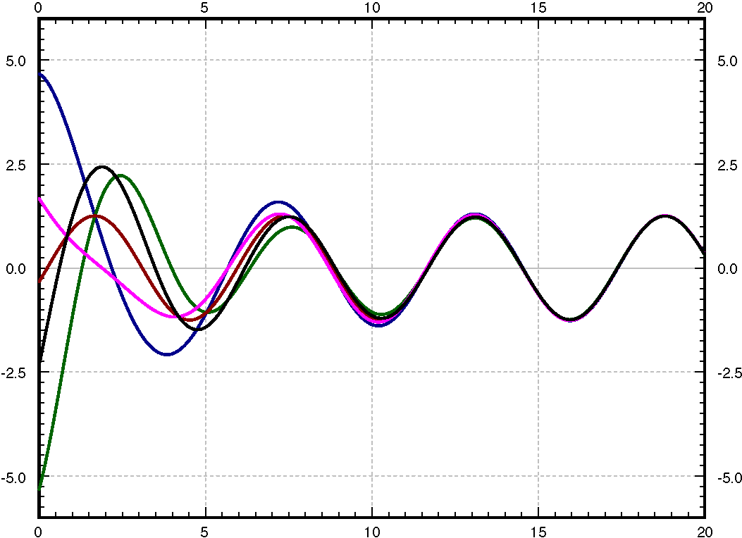
\begin{equation*} x = x_c + x_p = x_{tr} + x_{sp} . \end{equation*}

🔗

The transient solution $x_c = x_{tr}$ goes to zero as $t \to \infty\text{,}$ as all the terms involve an exponential with a negative exponent. So for large $t\text{,}$ the effect of $x_{tr}$ is negligible and we see essentially only $x_{sp}\text{.}$ Hence the name transient. Notice that $x_{sp}$ involves no arbitrary constants, and the initial conditions only affect $x_{tr}\text{.}$ Thus, the effect of the initial conditions is negligible after some period of time. We might as well focus on the steady periodic solution and ignore the transient solution. See Figure 2.6.8 for a graph given several different initial conditions.

🔗

The speed at which $x_{tr}$ goes to zero depends on $p$ (and hence $\gamma$). The bigger $p$ is (the bigger $\gamma$ is), the “faster” $x_{tr}$ becomes negligible. So the smaller the damping, the longer the “transient region” This is consistent with the observation that when $\gamma=0\text{,}$ the initial conditions affect the behavior for all time (i.e. an infinite “transient region”).

🔗

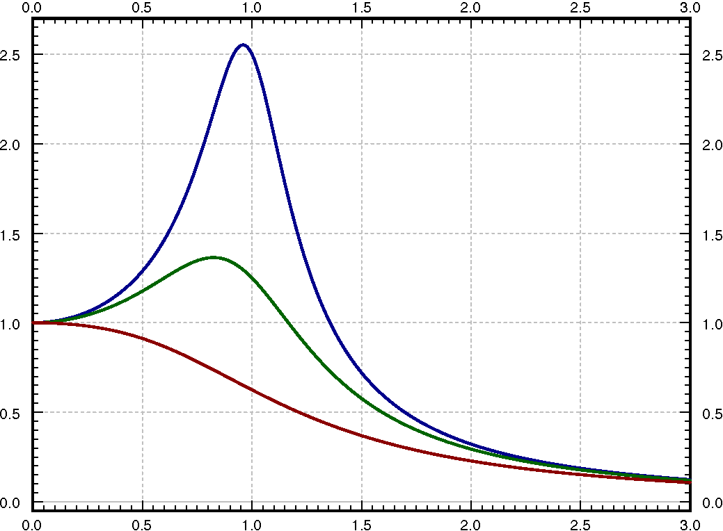
Let us describe what we mean by resonance when damping is present. Since there were no conflicts when solving with undetermined coefficient, there is no term that goes to infinity. We look instead at the maximum value of the amplitude of the steady periodic solution. Let $C$ be the amplitude of $x_{sp}\text{.}$ If we plot $C$ as a function of $\omega$ (with all other parameters fixed), we can find its maximum. We call the $\omega$ that achieves this maximum the practical resonance frequency. We call the maximal amplitude $C(\omega)$ the practical resonance amplitude. Thus when damping is present we talk of practical resonance rather than pure resonance. A sample plot for three different values of $\gamma$ is given in Figure 2.6.9. As you can see the practical resonance amplitude grows as damping gets smaller, and practical resonance can disappear altogether when damping is large.

🔗

The main takeaways from Figure 2.6.9 is that the amplitude can be larger than 1, which is the idea of resonance in this case. Based on Hooke’s law, we know that a constant force of magnitude $F_0$ will stretch (or compress) a spring with constant $k$ a length of $F_0/k\text{.}$ If we take $F_0 = 1$ and $k=1\text{,}$ as is done in Figure 2.6.9, then the resulting magnitude should be $1\text{.}$ However, if we don’t use a constant force of magnitude $F_0\text{,}$ but instead use an oscillatory force with frequency $\omega$ of the form $F(t) = F_0 \cos{(\omega t)}\text{,}$ we get an amplitude of $C(\omega)\text{.}$ This graph indicates how the forcing frequency changes the amplitude of the resulting oscillation. Since the amplitude “should” be $1$ based on $F_0/k\text{,}$ if $C(\omega) > 1\text{,}$ then the frequency chosen is causing an increase in the amplitude, which is the idea of practical resonance.

🔗

To find the maximum, or determine if there is a maximum, we need to find the derivative $C'(\omega)\text{.}$ Computation shows

\begin{equation*} C'(\omega) = \frac{- 2\omega( 2p^2+\omega^2-\omega_0^2)F_0} {m {\bigl({(2\omega p)}^2+{(\omega_0^2-\omega^2)}^2\bigr)}^{3/2}} . \end{equation*}

This is zero either when $\omega = 0$ or when $2p^2+\omega^2-\omega_0^2 = 0\text{.}$ In other words, $C'(\omega) = 0$ when

\begin{equation*} \mybxbg{ ~~ \omega = \sqrt{\omega_0^2 - 2p^2} \quad \text{or} \quad \omega = 0 . ~~ } \end{equation*}

If $\omega_0^2 - 2p^2$ is positive, then there is a positive value of $\omega\text{,}$ namely $\omega = \sqrt{\omega_0^2 - 2p^2}$ where the amplitude attains a maximum value. Since we know that the amplitude is $F_0/(m\omega_0^2)$ or $F_0/k$ when $\omega = 0\text{,}$ the maximum will be larger than this. As described above, this value, $F_0/k$ is the expected amplitude, that is, the amplitude you would get with no oscillation, so that if the amplitude is larger than this for some value of $\omega\text{,}$ this means that the oscillation at frequency $\omega$ is resonating with the system to create a larger oscillation. This is the idea of practical resonance. It is practical because there is damping, so the situation is more physically relevant (to contrast with pure resonance), and still results in larger amplitudes of oscillation.

🔗

Our previous work indicates that a system will exhibit practical resonance for some values of $\omega$ whenever $\omega_0^2 - 2p^2$ is positive, and the frequency where the amplitude hits the maximum value is at $\sqrt{\omega_0^2 - 2p^2}\text{.}$ This follows by the first derivative test for example as then $C'(\omega) > 0$ for small $\omega$ in this case. If on the other hand $\omega_0^2 - 2p^2$ is not positive, then $C(\omega)$ achieves its maximum at $\omega=0\text{,}$ and there is no practical resonance since we assume $\omega > 0$ in our system. In this case the amplitude gets larger as the forcing frequency gets smaller.

🔗

If practical resonance occurs, the peak frequency is smaller than $\omega_0\text{.}$ As the damping $\gamma$ (and hence $p$) becomes smaller, the peak practical resonance frequency goes to $\omega_0\text{.}$ So when damping is very small, $\omega_0$ is a good estimate of the peak practical resonance frequency. This behavior agrees with the observation that when $\gamma=0\text{,}$ then $\omega_0$ is the resonance frequency.

🔗

An infant is bouncing in a spring chair. The infant has a mass of kg, and the chair functions as a spring with spring constant . The bouncing of the infant applies a force of the form $6 \cos(\omega t)$ for some frequency $\omega\text{.}$ Assume that the infant starts at rest at the equilibrium position of the chair.

🔗

(a)

If there is no dampening coefficient, what frequency would the infant need to force at in order to generate pure resonance?

🔗

Answer.

$3$ rad/s or $\frac{3}{2\pi}$ Hz

🔗

(b)

Assume that the chair is built with a dampener with coefficient . Set up an initial value problem for this situation if the child acts in the same way as described in (a).

🔗

Answer.

$8y'' + 16y' + 72y = 6\cos(3t)\text{,}$ $y(0) = y'(0) = 0$

🔗

(c)

Solve this initial value problem.

🔗

Answer.

$y(t) = \frac{1}{8}\sin(3t) - \frac{3}{16\sqrt{2}}\sin(2\sqrt{2} t)$

🔗

(d)

There are several options for chairs you can buy. There is the one with dampening coefficient $\unitfrac[16]{Ns}{m}\text{,}$ one with $\unitfrac[1]{Ns}{m}\text{,}$ and one with $\unitfrac[30]{Ns}{m}\text{.}$ Which of these would be most ‘fun’ for the infant? How do you know?

🔗

Answer.

Assume that we have a mass-on-a-spring system defined by the equation

\begin{equation*} 3y'' + 2y' + 18y = 4\cos(5t). \end{equation*}

🔗

(a)

Identify the mass, dampening coefficient, and spring constant for the system.

🔗

Answer.

$m = 3$ kg, $\gamma = 2$ Ns/m, $k = 18$ N/m

🔗

(b)

Use the entire equation to find the natural frequency, forcing frequency, and quasi-frequency of this oscillation.

🔗

Answer.

Natural is $\sqrt{6}$ rad/s, Forcing is $5$ rad/s, Quasi-frequency is $\frac{\sqrt{53}}{3}$ rad/s

🔗

(c)

Two of these frequencies will show up in the general solution to this problem. Which are they, and in which part (transient, steady-periodic) do they appear?

🔗

Answer.

Quasifrequency is in the transient, and forcing is in steady periodic.

🔗

(d)

Find the general solution of this problem.

🔗

Answer.

$C_1e^{-t/3}\cos\left(\frac{\sqrt{53}}{3}t\right) + C_2e^{-t/3}\sin\left(\frac{\sqrt{53}}{3}t\right) - \frac{228}{3349} \cos(5t) + \frac{40}{3349}\sin(5t)$

🔗

15.

A circuit is built with an $L$ Henry inductor, and $R$ Ohm resistor, and a $C$ Farad capacitor. All of the units are correct, but you do not know any of their values. To study this circuit, you apply an external voltage source of $F(t) = 4 \cos\left(\frac{1}{2} t \right)\text{,}$ and the circuit starts with no initial charge or current.

🔗

(a)

Write an initial value problem to model this situation.

🔗

Answer.

$LQ'' + RQ' + \frac{1}{C}Q = 4\cos\left(\frac{1}{2}t\right)$

🔗

(b)

Your friend (who knows more about this circuit than you do) takes a reading from this circuit after it is running and says “The amplitude of the charge oscillation is greater than 100 coulombs, which means this circuit is exhibiting practical resonance.” There are three facts that you can learn about this circuit from the statement here that will tell you about the values of $L\text{,}$ $R\text{,}$ and $C\text{.}$

This statement seems to imply that the expected amplitude of the oscillation is 100 coulombs. What does this mean about the value of $C\text{?}$
🔗

🔗
Your friend says that this circuit is in practical resonance. What does this tell you about the value of $R$ in this case?
🔗

🔗
Finally, being in practical resonance says something about how the forcing frequency compares to the natural frequency of this system. What is that, and how does it relate to the value of $L\text{?}$
🔗

🔗

🔗

Answer.

$C = 25$ F
🔗

🔗
$R > 0$ but small
🔗

🔗
$\displaystyle L \approx \frac{4}{25}$
🔗

🔗

🔗

(c)

What is the frequency of the steady-periodic oscillation that your friend mentioned above?

🔗

Answer.

$\frac{1}{2}$

🔗

Prev Top Next