In the last three sections, we looked at the different options for two-component constant-coefficient systems. We want to determine a nice way to put all of this together. We summarize the behavior of linear homogeneous two-dimensional systems given by a nonsingular matrix in Table 4.7.1. Systems where one of the eigenvalues is zero (the matrix is singular) come up in practice from time to time, see Example 4.1.2, and the pictures are somewhat different (simpler in a way). See the exercises.
The sketches of all of these different behaviors and phase portraits can be found in their respective sections. Make sure that you understand the terminology, general behavior, and sketches for each of these different cases.
One other way to interpret and analyze this information is using the trace and determinant of the matrix. Recall from Section 3.6 that the trace of a matrix is the sum of the diagonal entries of the matrix and the determinant of the matrix is computed from the entries and is a way to determine invertibility of the matrix. If we take a generic \(2 \times 2\) matrix and find the characteristic polynomial, we get that for
\begin{equation*}
A = \begin{bmatrix} a & b \\ c & d \end{bmatrix},
\end{equation*}
A lot depends on the value of \(T^2 - 4D\text{.}\) If \(T^2 - 4D > 0,\) then we will have two real distinct eigenvalues. If \(T^2 - 4D = 0,\) then there is a single repeated eigenvalue, and if \(T^2 - 4D < 0\text{,}\) we have complex eigenvalues.
If \(D < 0\text{,}\) then \(T^2 - 4D > T^2,\) which means that \(\sqrt{T^2 - 4D} > |T|\text{.}\) If we put this into (4.7.1), this will mean that the term that is after the \(\pm\) will be larger than \(T\) in absolute value. Therefore, the two eigenvalues will be real and have opposite signs.
If \(D \geq 0\text{,}\) then the sign of the eigenvalues, or the sign of the real part in the complex case, is dictated by the sign of \(T\text{.}\) If \(D \geq 0\text{,}\) then \(T^2 - 4D \leq T^2\text{,}\) so that the part under the square root in (4.7.1) is always smaller in absolute value than \(T\text{.}\) Thus, both the plus and minus version will have values that are the same sign as \(T\text{.}\) If the expression is complex, then the real part is exactly \(T/2\text{,}\) which is the same sign as \(T\text{.}\)
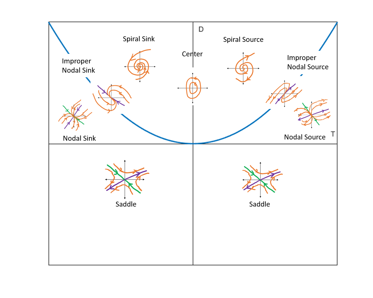
Since these are all based on the relation between \(T\) and \(D\text{,}\) we can also combine all of this into a figure to summarize the details. In Figure 4.7.3, \(T\) is on the horizontal axis and \(D\) is the vertical axis. The graph drawn is \(D = \nicefrac{T^2}{4}\text{,}\) which is the important criteria that shows up in the table.
Figure 4.7.3 can be used to determine the behavior of a two-component system without actually needing to solve the differential equation. The point is that the signs and type of the eigenvalues determine the structure of the solution, and we can determine the important qualities of these using just the trace and determinant of a matrix.
From the matrix, we can see that the trace is \(1 + 3 = 4\) and the determinant is \((1)(3) - (4)(-2) = 11\text{.}\) We see that \(D > 0\) with \(T^2 = 16\) and \(4D = 44 > 16\text{.}\) Therefore, we have \(4D > T^2\text{,}\) so we are above the curve on the graph, and so have a spiral. Since \(T > 0\text{,}\) this will be a spiral source.
Note: If you wanted to get a general solution or sketch a phase portrait for this differential equation, you would need to actually solve it out for that; you can not get enough information just from this image to sketch a proper phase portrait.
Compute the eigenvalues for the system above, find the general solution, and verify that this is a spiral source. The numbers here will not work out great, so having the quick analysis that it is a spiral source is nice.
What happens in the case when \(P =
\left[ \begin{smallmatrix} 1 & 1 \\ 0 & 1 \end{smallmatrix} \right]\text{?}\) In this case the eigenvalue is repeated and there is only one independent eigenvector. What picture does this look like?
What happens in the case when \(P =
\left[ \begin{smallmatrix} 1 & 1 \\ 1 & 1 \end{smallmatrix} \right]\text{?}\) Does this look like any of the pictures we have drawn?
Which behaviors are possible if \(P\) is diagonal, that is \(P = \left[ \begin{smallmatrix} a & 0 \\ 0 & b \end{smallmatrix} \right]\text{?}\) You can assume that \(a\) and \(b\) are not zero.
For each of the following matrices \(A\text{,}\) describe the behavior and classify the phase portrait of the system given by \({\vec{x}}' = A\vec{x}\text{.}\) Use the eigenvalues to determine this.
Take the system from Example 4.1.2, \(x_1'=\frac{r}{V}(x_2-x_1)\text{,}\)\(x_2'=\frac{r}{V}(x_1-x_2)\text{.}\) As we said, one of the eigenvalues is zero. What is the other eigenvalue, how does the picture look like and what happens when \(t\) goes to infinity.
Take \(\left[ \begin{smallmatrix}
x \\ y
\end{smallmatrix}\right] '
=
\left[ \begin{smallmatrix}
0 & 1 \\ 0 & 0
\end{smallmatrix}\right]
\left[ \begin{smallmatrix}
x \\ y
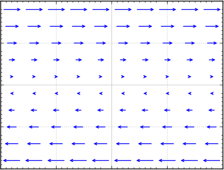
\end{smallmatrix}\right]\text{.}\) Draw the vector field and describe the behavior. Is it one of the behaviors that we have seen before?
Figure4.7.6.Vector field for the system \(\left[ \begin{smallmatrix}
x \\ y
\end{smallmatrix}\right] '
=
\left[ \begin{smallmatrix}
0 & 1 \\ 0 & 0
\end{smallmatrix}\right]
\left[ \begin{smallmatrix}
x \\ y
\end{smallmatrix}\right]\text{.}\)
The solution does not move anywhere if \(y = 0\text{.}\) When \(y\) is positive, the solution moves (with constant speed) in the positive \(x\) direction. When \(y\) is negative, the solution moves (with constant speed) in the negative \(x\) direction. It is not one of the behaviors we have seen.
Note that the matrix has a double eigenvalue 0 and the general solution is \(x = C_1 t + C_2\) and \(y = C_1\text{,}\) which agrees with the description above.
In this exercise, we will analyze “perturbations” or near-by matrices to the ones that are given. This will be important later in Section 5.1. For each of the following matrices
Find the trace and determinant, and use them to classify the behavior of the linear system \({\vec{x}}' = A\vec{x}\) for the given matrix \(A\text{.}\)
Draw a sketch of the trace-determinant plane, including the curve \(D = \nicefrac{T^2}{4}\text{,}\) and plot the point corresponding to the matrix on those axes.
Look at the points in a small (as small as you want) circle around the point you just drew. What does the behavior look like for systems whose matrices fall within that circle? What do these behaviors have in common with each other, and how do they differ?
\(T = 0\text{,}\)\(D = 1\text{.}\) Center. Points nearby are all spirals, but they could be asymptotically stable, centers, or unstable. Stability is unknown.
\(T = -8\text{,}\)\(D = 16\text{.}\) Improper nodal sink. All points nearby will be asymptotically stable, but they could be nodal sinks, improper nodal sinks, or spiral sinks.
\(T = 2\text{,}\)\(D = 1\text{.}\) Improper nodal source. All points nearby will be unstable, but they may be spirals, nodal sources, or improper nodal sources.