Section 1.3 Separable equations

As mentioned in SectionΒ 1.1, when a differential equation is of the form \(y' = f(x)\text{,}\) we can just integrate: \(y = \int f(x) \,dx + C\text{.}\) Unfortunately this method no longer works for the general form of the equation \(y' = f(x,y)\text{.}\) Integrating both sides yields
\begin{equation*} y = \int f(x,y) \, dx + C\text{.} \end{equation*}
Notice the dependence on \(y\) in the integral. Since \(y\) is a function of \(x\text{,}\) this expression is really of the form
\begin{equation*} y = \int f(x, y(x))\, dx + C \end{equation*}
and without knowing what \(y(x)\) is in advance (which we don’t, because that’s what we are trying to solve for) we can’t compute this integral. Note that while you may have seen integrals of the form
\begin{equation*} \int f(x,y)\, dx \end{equation*}
in Calculus 3, this is not the same situation. In that class, \(x\) and \(y\) were both independent variables, so we could integrate this expression in \(x\text{,}\) treating \(y\) as a constant. However, here \(y\) is a function of \(x\text{,}\) so they are not both independent variables and \(y\) can not be treated like a constant. If \(y\) is a function of \(x\) and any \(y\) shows up in the integral, you can not compute it.

Subsection Separable equations

One particular type of differential equation that we can evaluate using a technique very similar to direct integration is separable equations.

Definition 1.3.1.

We say a differential equation is separable if we can write it as
\begin{equation*} y' = f(x)g(y)\text{,} \end{equation*}
for some functions \(f(x)\) and \(g(y)\text{.}\)
Let us write the equation in Leibniz Notation
\begin{equation*} \frac{dy}{dx} = f(x)g(y)\text{.} \end{equation*}
Then we rewrite the equation as
\begin{equation*} \frac{dy}{g(y)} = f(x) \,dx\text{.} \end{equation*}
It looks like we just separated the derivative as a fraction. The actual reasoning here is the differential from Calculus 1. This is the fact that for \(y\) a function of \(x\text{,}\) we know that
\begin{equation*} dy = \frac{dy}{dx} dx\text{.} \end{equation*}
This means that we can take the equation
\begin{equation*} \frac{dy}{dx} = f(x)g(y)\text{,} \end{equation*}
rearrange it as
\begin{equation*} \frac{1}{g(y)} \frac{dy}{dx} = f(x) \end{equation*}
and then multiply both sides by \(dx\) to get
\begin{equation*} \frac{1}{g(y)} \frac{dy}{dx}\ dx = f(x) dx \end{equation*}
which leads to the rewritten equation above. Both sides look like something we can integrate. We obtain
\begin{equation*} \int \frac{dy}{g(y)} = \int f(x) \,dx + C\text{.} \end{equation*}
If we can find closed form expressions for these two integrals, we can, perhaps, solve for \(y\text{.}\)

Example 1.3.2.

Solve the equation
\begin{equation*} y' = xy\text{.} \end{equation*}
Solution.
Note that \(y=0\) is a solution. We will remember that fact and assume \(y \not =0\) from now on, so that we can divide by \(y\text{.}\) Write the equation as \(\frac{dy}{dx} = xy\text{.}\) Then
\begin{equation*} \int \frac{dy}{y} = \int x\,dx + C\text{.} \end{equation*}
We compute the antiderivatives to get
\begin{equation*} \ln \, \lvert y\rvert = \frac{x^2}{2} + C\text{,} \end{equation*}
or
\begin{equation*} \lvert y \rvert = e^{\frac{x^2}{2} + C} = e^{\frac{x^2}{2}} e^C = D e^{\frac{x^2}{2}}\text{,} \end{equation*}
where \(D > 0\) is some constant. Because \(y=0\) is also a solution and because of the absolute value we can write:
\begin{equation*} y = D e^{\frac{x^2}{2}}\text{,} \end{equation*}
for any number \(D\) (including zero or negative).
We check:
\begin{equation*} y' = D x e^{\frac{x^2}{2}} = x \left( D e^{\frac{x^2}{2}} \right) = xy\text{.} \end{equation*}
Yay!
One particular case in which this method works very well is if the function \(f(x,y)\) is only a function of \(y\text{.}\) With this, we can explicitly complete the solution to equations like
\begin{equation*} y' = ky\text{.} \end{equation*}
reaching the solution \(y(x) = e^{kx}\text{.}\)
We should be a little bit more careful with this method. You may be worried that we integrated in two different variables. We seemingly did a different operation to each side. Let us work through this method more rigorously. Take
\begin{equation*} \frac{dy}{dx} = f(x)g(y)\text{.} \end{equation*}
We rewrite the equation as follows. Note that \(y = y(x)\) is a function of \(x\) and so is \(\frac{dy}{dx}\text{!}\)
\begin{equation*} \frac{1}{g(y)}\,\frac{dy}{dx} = f(x)\text{.} \end{equation*}
We integrate both sides with respect to \(x\text{:}\)
\begin{equation*} \int \frac{1}{g(y)}\,\frac{dy}{dx} \,dx = \int f(x) \,dx + C\text{.} \end{equation*}
We use the change of variables formula (substitution) on the left hand side:
\begin{equation*} \int \frac{1}{g(y)}\,dy = \int f(x) \,dx + C\text{.} \end{equation*}
And we are done.
However, in some cases there are some special solutions to these problems as well that don’t fit the same formula. Assume we have
\begin{equation*} \frac{dy}{dx} = f(x)g(y) \end{equation*}
and we have a value \(y_0\) such that \(g(y_0) = 0\text{.}\) Then, the function \(y(x) = y_0\) is a solution, provided \(f(x)\) is defined everywhere. (Plug this in and check!) This fills in the issue for having \(\frac{1}{g(y)}\) in our integral expression, which is not defined when \(g(y) = 0\text{.}\) These are called singular solutions, and the next example will showcase one of them.

Subsection Implicit solutions

We sometimes get stuck even if we can do the integration. Consider the separable equation
\begin{equation*} y' = \frac{xy}{y^2+1} . \end{equation*}
We separate variables,
\begin{equation*} \frac{y^2+1}{y}\,dy = \left(y+\frac{1}{y}\right)\,dy = x\,dx\text{.} \end{equation*}
We integrate to get
\begin{equation*} \frac{y^2}{2} + \ln \, \lvert y \rvert = \frac{x^2}{2} + C\text{,} \end{equation*}
or perhaps the easier looking expression (where \(D = 2C\))
\begin{equation*} y^2 + 2 \ln \, \lvert y\rvert = x^2 + D\text{.} \end{equation*}
It is not easy to find the solution explicitly as it is hard to solve for \(y\text{.}\) We, therefore, leave the solution in this form and call it an implicit solution. It is still easy to check that an implicit solution satisfies the differential equation. In this case, we differentiate with respect to \(x\text{,}\) and remember that \(y\) is a function of \(x\text{,}\) to get
\begin{equation*} y'\left(2y + \frac{2}{y}\right) = 2x\text{.} \end{equation*}
Multiply both sides by \(y\) and divide by \(2(y^2+1)\) and you will get exactly the differential equation. We leave this computation to the reader.
If you have an implicit solution, and you want to compute values for \(y\text{,}\) you might have to be tricky. You might get multiple solutions \(y\) for each \(x\text{,}\) so you have to pick one. Sometimes you can graph \(x\) as a function of \(y\text{,}\) and then flip your paper. Sometimes you have to do more.
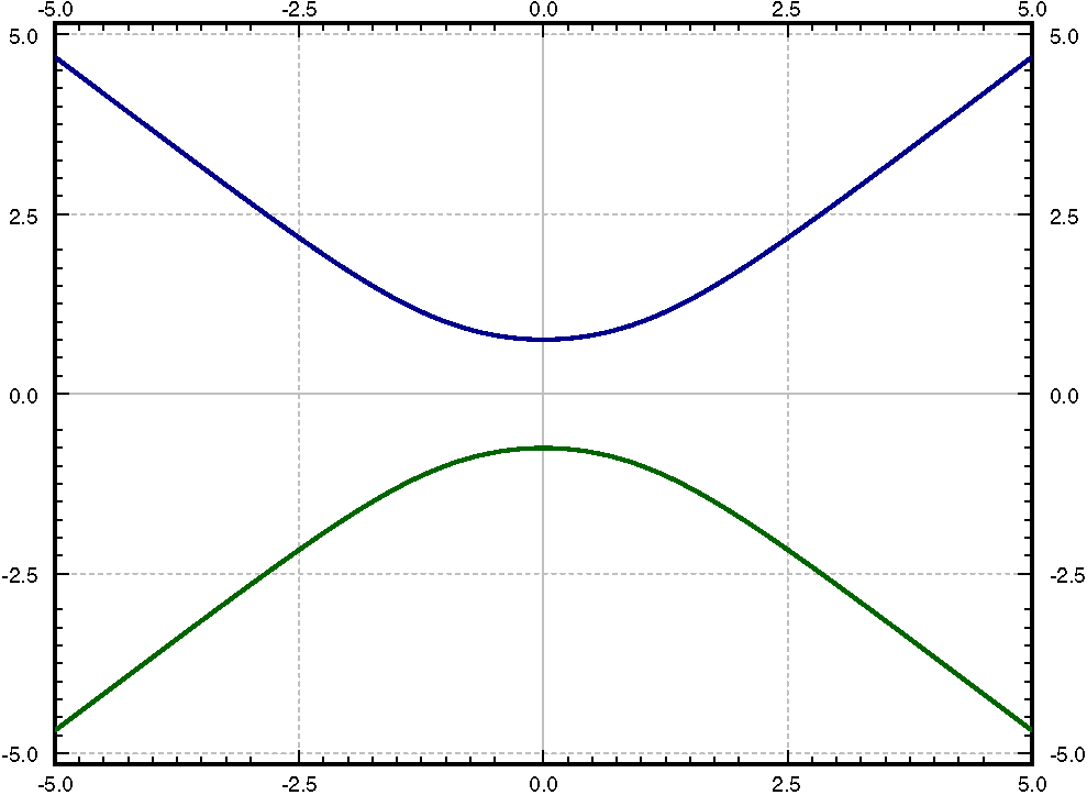
Computers are also good at some of these tricks. More advanced mathematical software usually has some way of plotting solutions to implicit equations, which makes these solutions just as good for visualizing or graphing as explicit solutions. For example, for \(C=0\) if you plot all the points \((x,y)\) that are solutions to \(y^2+2\ln|y|=x^2\text{,}\) you find the two curves in FigureΒ 1.3.3. This is not quite a graph of a function. For each \(x\) there are two choices of \(y\text{.}\) To find a function you would have to pick one of these two curves. You pick the one that satisfies your initial condition if you have one. For example, the top curve satisfies the condition \(y(1)=1\text{.}\) So for each \(C\) we really got two solutions. As you can see, computing values from an implicit solution can be somewhat tricky, but sometimes, an implicit solution is the best we can do.
A graph showing two curves, both representing the same implicit solution. The graph is somewhat parabolic, one pointing up and one pointing down.
The graph shows two different curves, both composing the implicit solution \(y^2 + 2\ln\lvert y \rvert = x^2\text{.}\) One comes in from the top left, coming to a minimum at \(x=0\) and then leaving to the top right. The second curve comes in from the bottom left, hits a maximum at \(x=0\) and then leaves to the bottom right.
Figure 1.3.3. The implicit solution \(y^2 + 2\ln\lvert y \rvert = x^2\) to \(y' = \frac{xy}{y^2 + 1}\text{.}\)
The equation above also has the solution \(y=0\text{.}\) Since our function
\begin{equation*} g(y) = \frac{y}{y^2 + 1} \end{equation*}
is zero at \(y=0\text{,}\) and gives an additional solution to the problem. The function \(y(x) = 0\) satisfies \(y'(x) = 0\) and \(\frac{xy}{y^2 + 1} = 0\) for all \(x\text{,}\) which is the right-hand side of the equation. So the general solution is
\begin{equation*} y^2 + 2 \ln \, \lvert y \rvert = x^2 + C, \qquad \text{and} \qquad y=0. \end{equation*}
These outlying solutions such as \(y=0\) are sometimes called singular solutions, as mentioned previously.

Subsection Examples of separable equations

Example 1.3.4.

Solve \(x^2y' = 1 - x^2+y^2 - x^2y^2\text{,}\) \(y(1) = 0\text{.}\)
Solution.
Factor the right-hand side
\begin{equation*} x^2y' = (1 - x^2)(1+y^2)\text{.} \end{equation*}
Separate variables, integrate, and solve for \(y\text{:}\)
\begin{align*} \frac{y'}{1+y^2} \amp = \frac{1 - x^2}{x^2}\\ \frac{y'}{1+y^2} \amp = \frac{1}{x^2} - 1 \\ \operatorname{arctan} (y) \amp = \frac{-1}{x} - x + C\\ y \amp = \tan \left(\frac{-1}{x} - x + C\right) \end{align*}
Solve for the initial condition, \(0 = \tan(-2+C)\) to get \(C=2\) (or \(C = 2 + \pi\text{,}\) or \(C = 2 + 2\pi\text{,}\) etc.). The particular solution we seek is, therefore,
\begin{equation*} y = \tan \left(\frac{-1}{x} - x + 2 \right)\text{.} \end{equation*}

Example 1.3.5. A first modeling problem.

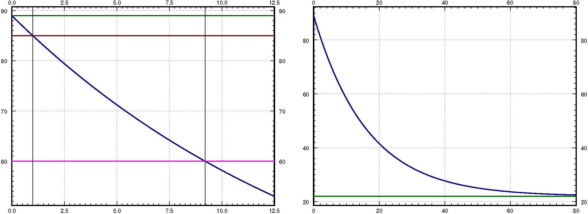
Bob made a cup of coffee, and Bob likes to drink coffee only once reaches 60 degrees Celsius and will not burn him. Initially at time \(t=0\) minutes, Bob measured the temperature and the coffee was 89 degrees Celsius. One minute later, Bob measured the coffee again and it had 85 degrees. The temperature of the room (the ambient temperature) is 22 degrees. When should Bob start drinking?
Solution.
Let \(T\) be the temperature of the coffee in degrees Celsius, and let \(A\) be the ambient (room) temperature, also in degrees Celsius. Newton’s Law of Cooling states that the rate at which the temperature of the coffee is changing is proportional to the difference between the ambient temperature and the temperature of the coffee. That is,
\begin{equation*} \frac{dT}{dt} = k(A-T) , \end{equation*}
for some constant \(k\text{.}\) For our setup \(A=22\text{,}\) \(T(0) = 89\text{,}\) \(T(1) = 85\text{.}\) We separate variables and integrate (let \(C\) and \(D\) denote arbitrary constants):
\begin{align*} \frac{1}{T-A} \, \frac{dT}{dt} & = -k \\ \ln (T-A) &= -kt + C , \qquad \text{(note that } T-A > 0 \text{)} \\ T-A &= D\, e^{-kt} \\ T &= A + D\, e^{-kt} \text{.} \end{align*}
That is, \(T = 22 + D\, e^{-kt}\text{.}\) We plug in the first condition: \(89 = T(0) = 22 + D\text{,}\) and hence \(D = 67\text{.}\) So \(T = 22 + 67\, e^{-kt}\text{.}\) The second condition says \(85 = T(1) = 22 + 67\, e^{-k}\text{.}\) Solving for \(k\) we get \(k = - \ln \frac{85-22}{67} \approx 0.0616\text{.}\) Now we solve for the time \(t\) that gives us a temperature of 60 degrees. Namely, we solve
\begin{equation*} 60 = 22 + 67 e^{-0.0616t} \end{equation*}
to get \(t = - \frac{\ln\frac{60-22}{67}}{0.0616} \approx 9.21\) minutes. So Bob can begin to drink the coffee at just over 9 minutes from the time Bob made it. That is probably about the amount of time it took us to calculate how long it would take. See FigureΒ 1.3.6.
described in detail following the image
The left graph shows the decaying temperature of the coffee over the time range of 0 to 12.5 minutes, with markings for 89, 85, and 60 degrees as described in the caption. The plot on the right shows the same curve over the range of 0 to 90 minutes to show the long-time behavior approaching 22.
Figure 1.3.6. Graphs of the coffee temperature function \(T(t)\text{.}\) On the left, horizontal lines are drawn at temperatures 60, 85, and 89. Vertical lines are drawn at \(t=1\) and \(t=9.21\text{.}\) Notice that the temperature of the coffee hits 85 at \(t=1\text{,}\) and 60 at \(t \approx 9.21\text{.}\) On the right, the graph is over a longer period of time, with a horizontal line at the ambient temperature 22.

Example 1.3.7. Example with singular solutions.

Find the general solution to \(y' = \frac{-xy^2}{3}\) (including singular solutions).
Solution.
First note that \(y=0\) is a solution (a singular solution). Now assume that \(y \not= 0\text{.}\)
\begin{align*} \frac{-3}{y^2} y' & = x\\ \frac{3}{y} & = \frac{x^2}{2} + C\\ y & = \frac{3}{\frac{x^2}{2} + C}= \frac{6}{x^2 + 2C} \text{.} \end{align*}
So the general solution is,
\begin{equation*} y = \frac{6}{x^2 + 2C}, \qquad \text{and} \qquad y=0\text{.} \end{equation*}

Example 1.3.8.

Find the general solution to
\begin{equation*} \frac{dy}{dx} = (x^2 + e^x)(y^2 - 3y - 4). \end{equation*}
Solution.
Using the methods of separable equations, we can rewrite this differential equation as
\begin{equation*} \frac{dy}{y^2 - 3y - 4} = (x^2 + e^x) \ dx \end{equation*}
and we can integrate both sides to solve. This leads to
\begin{equation*} \int \frac{dy}{y^2 - 3y + 4} = \int x^2 + e^x\ dx. \end{equation*}
The right-hand side of this can be integrated normally to give
\begin{equation*} \int x^2 + e^x\ dx = \frac{x^3}{3} + e^x + C \end{equation*}
and the left-hand side requires partial fractions in order to integrate correctly. If you are not familiar with this technique of partial fractions, it is reviewed in SectionΒ A.3.
Using the method of partial fractions, we want to rewrite
\begin{equation*} \frac{1}{y^2 - 3y - 4} = \frac{A}{y-4} + \frac{B}{y+1} \end{equation*}
and solve for \(A\) and \(B\text{,}\) which gives
\begin{equation*} \frac{1}{y^2 - 3y - 4} = \frac{1/5}{y-4} - \frac{1/5}{y+1}. \end{equation*}
Therefore, we can compute the integral
\begin{align*} \int \frac{dy}{y^2 - 3y - 4} \amp = \int \frac{1/5}{y-4} - \frac{1/5}{y+1} dy \\ \amp = \frac{1}{5} \ln(|y-4|) - \frac{1}{5} \ln(|y+1|) + C\text{.} \end{align*}
Therefore, we can write the general solution as
\begin{equation*} \frac{1}{5} \ln{\left(\frac{|y-4|}{|y+1|} \right)} = \frac{x^3}{3} + e^x + C. \end{equation*}
We could solve this out for \(y\) as an explicit function, but that is not necessary for a problem like this.
There are also two singular solutions here at \(y=4\) and \(y=-1\text{.}\) Notice that the implicit solution that we found previously is not defined at either of these values, because they involve taking the natural log of \(0\text{,}\) which is not defined.
Exercises Exercises

3.

Solve \(y' = (y-1)(y+1)\) for \(y(0)=3\text{.}\) (Note: Requires partial fractions)
Answer.
\(y = \frac{2 + e^{2t}}{2 - e^{2t}}\)

8.

Consider the differential equation
\begin{equation*} \frac{dy}{dx} = \frac{2x}{y} \end{equation*}
(b)
Find the solution to this differential equation as an explicit function with \(y(1) = 4\text{.}\)
Answer.
\(y = \sqrt{2x^2 + 14}\)
(c)
Find the solution to this differential equation as an explicit function with \(y(0) = -2\text{.}\)
Answer.
\(y = -\sqrt{2x^2 + 4}\)

9.

Solve \(y' = y^n\text{,}\) \(y(0) = 1\text{,}\) where \(n\) is a positive integer. Hint: You have to consider different cases.
Answer.
If \(n \neq 1\text{,}\) then \(y={\bigl((1-n)x+1\bigr)}^{1/(1-n)}\text{.}\) If \(n=1\text{,}\) then \(y = e^x\text{.}\)

10.

Solve \(\dfrac{dx}{dt} = (x^2-1)\,t\text{,}\) for \(x(0) = 0\text{.}\) (Note: Requires partial fractions)
Answer.
\(x = \frac{1 - e^{t^2}}{1 + e^{t^2}}\)

16.

Find the general solution of \(y' = e^x\text{,}\) and then \(y' = e^y\text{.}\)
Answer.
\(y = e^x + C\text{,}\) \(y= -\ln(|-x-C|)\)

19.

Solve \(\dfrac{dy}{dx} = \dfrac{y^2+1}{x^2+1}\text{,}\) for \(y(0) = 1\text{.}\)
Answer.
\(y = \tan\left(\tan^{-1}(x) + \frac{\pi}{4}\right)\)

20.

Find an implicit solution for \(\dfrac{dy}{dx} = \dfrac{x^2+1}{y^2+1}\text{,}\) for \(y(0) = 1\text{.}\)
Answer.
\(\frac{y^3}{3} + y = \frac{x^3}{3} + x + \frac{4}{3}\)

22.

Find an implicit solution for \(xy' = \frac{x^2 + 1}{y^2 - 1}\) with \(y(3) = 2\text{.}\)
Answer.
\(\frac{y^3}{3} - y = \frac{x^2}{2} +\ln(|x|) + 4 - \ln(2)\)

23.

Find an explicit solution for \(y' = xe^{-y}\text{,}\) \(y(0)=1\text{.}\)
Answer.
\(y = \ln\left(\frac{x^2}{2} + e \right)\)

26.

Find an explicit solution for \(y' = y^2(x^4 + 1)\) with \(y(1) = 2\text{.}\)
Answer.
\(y = \frac{1}{\frac{17}{10} - x - \frac{x^5}{5}}\)

27.

Find an explicit solution for \(y' = \frac{\cos(x)+ 1}{y}\) with \(y(0) = 4\) .
Answer.
\(y = \sqrt{2\sin(x) + 2x + 16}\)

28.

Find an explicit solution for \(y' = ye^{-x^2}\text{,}\) \(y(0)=1\text{.}\) It is alright to leave a definite integral in your answer.
Answer.
\(y = e^{\int_0^x e^{-s^2}\ ds}\)

30.

Is the equation \(y' = ty^2 + t\) separable? If so, find the general solution, if not, explain why.
Answer.
Yes. \(y = \tan\left(\frac{t^2}{2} + C\right)\)

31.

Is the equation \(y' = xy^2 + 3y^2 - 4x - 12\) separable? If so, find the general solution, if not, explain why. (Note: Requires partial fractions)
Answer.
Yes. \(\frac{1}{2\sqrt{3}}\ln\left(\left| \frac{y - \sqrt{3}}{y+\sqrt{3}}\right|\right) = \frac{x^2}{2} + 3x + C\)

32.

Suppose a cup of coffee is at 100 degrees Celsius at time \(t=0\text{,}\) it is at 70 degrees at \(t=10\) minutes, and it is at 50 degrees at \(t=20\) minutes. Compute the ambient temperature.
Answer.

33.

Take ExampleΒ 1.3.5with the same numbers: 89 degrees at \(t=0\text{,}\) 85 degrees at \(t=1\text{,}\) and ambient temperature of 22 degrees. Suppose these temperatures were measured with precision of \(\pm 0.5\) degrees. Given this imprecision, the time it takes the coffee to cool to (exactly) 60 degrees is also only known in a certain range. Find this range. Hint: Think about what kind of error makes the cooling time longer and what shorter.
Answer.
The range is approximately 7.45 to 12.15 minutes.

34.

A population \(x\) of rabbits on an island is modeled by \(x' = x- \bigl(\frac{1}{1000} \bigr) x^2\text{,}\) where the independent variable is time in months. At time \(t=0\text{,}\) there are 40 rabbits on the island.
(b)
How many rabbits are on the island in 1 month, 5 months, 10 months, 15 months (round to the nearest integer).
Answer.
102 rabbits after one month, 861 after 5 months, 999 after 10 months, 1000 after 15 months.