If the equation can be solved in closed form, we should do that. But what if we have an equation that cannot be solved in closed form? What if we want to find the value of the solution at some particular \(x\text{?}\) Or perhaps we want to produce a graph of the solution to inspect the behavior. In this section we will learn about the basics of numerical approximation of solutions.
The simplest method for approximating a solution is Euler’s Method 1
Named after the Swiss mathematician Leonhard Paul Euler (1707-1783). The correct pronunciation of the name sounds more like "oiler"
. It works as follows: Take \(x_0\) and compute the slope \(k = f(x_0,y_0)\text{.}\) The slope is the change in \(y\) per unit change in \(x\text{.}\) Follow the line for an interval of length \(h\) on the \(x\)-axis. Hence if \(y = y_0\) at \(x_0\text{,}\) then we say that \(y_1\) (the approximate value of \(y\) at \(x_1 = x_0 + h\)) is \(y_1 = y_0
+ h k\text{.}\) Rinse, repeat! Let \(k = f(x_1,y_1)\text{,}\) and then compute \(x_2 = x_1 + h\text{,}\) and \(y_2 = y_1 + h k\text{.}\) Now compute \(x_3\) and \(y_3\) using \(x_2\) and \(y_2\text{,}\) etc. Consider the equation \(y' = \nicefrac{y^2}{3}\text{,}\)\(y(0)=1\text{,}\) and \(h=1\text{.}\) Then \(x_0=0\) and \(y_0 = 1\text{.}\) We compute
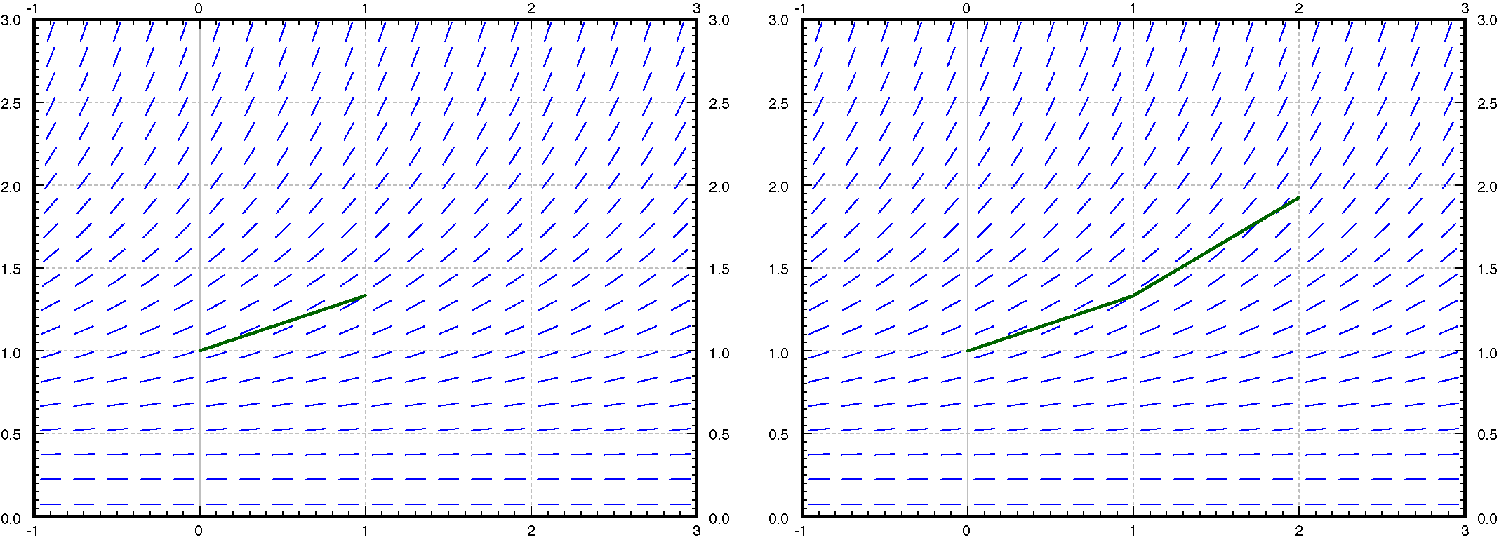
We then draw an approximate graph of the solution by connecting the points \((x_0,y_0)\text{,}\)\((x_1,y_1)\text{,}\)\((x_2,y_2)\text{,}\)…. For the first two steps of the method see Figure 1.6.1.
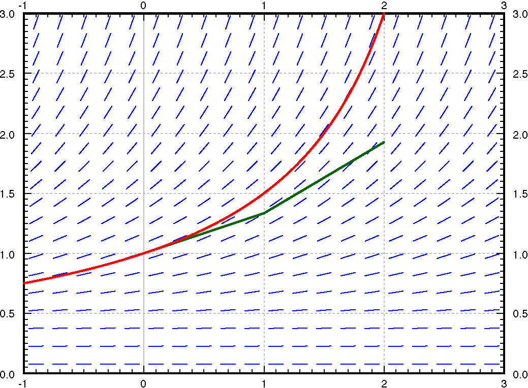
This can be worked out by hand for a few steps, but the formulas here lend themselves very well to being coded into a looping structure for more involved processes. The line segments we get are an approximate graph of the solution. Generally it is not exactly the solution. See Figure 1.6.2 for the plot of the real solution and the approximation.
Figure1.6.2.Two steps of Euler’s method (step size 1) and the exact solution for the equation \(y' = \frac{y^2}{3}\) with initial conditions \(y(0)=1\text{.}\)
We continue with the equation \(y' = \nicefrac{y^2}{3}\text{,}\)\(y(0)=1\text{.}\) Let us try to approximate \(y(2)\) using Euler’s method. In Figure 1.6.1 and Figure 1.6.2 we have graphically approximated \(y(2)\) with step size 1. With step size 1, we have \(y(2) \approx 1.926\text{.}\) The real answer is 3. We are approximately 1.074 off. Let us halve the step size. Computing \(y_4\) with \(h=0.5\text{,}\) we find that \(y(2) \approx 2.209\text{,}\) so an error of about 0.791. Table 1.6.4 gives the values computed for various parameters.
The difference between the actual solution and the approximate solution is called the error. We usually talk about just the size of the error and we do not care much about its sign. The point is, we usually do not know the real solution, so we only have a vague understanding of the error. If we knew the error exactly …what is the point of doing the approximation?
Notice that except for the first few times, every time we halved the step size the error approximately halved. This halving of the error is a general feature of Euler’s method as it is a first order method. There exists an improved Euler method, see the exercises, which is a second order method. A second order method reduces the error to approximately one quarter every time we halve the interval. The meaning of "second" order is the squaring in \(\nicefrac{1}{4} = \nicefrac{1}{2}
\times
\nicefrac{1}{2} = {(\nicefrac{1}{2})}^2\text{.}\)
To get the error to be within 0.1 of the answer we had to already do 64 steps. To get it to within 0.01 we would have to halve another three or four times, meaning doing 512 to 1024 steps. That is quite a bit to do by hand. The improved Euler method from the exercises should quarter the error every time we halve the interval, so we would have to approximately do half as many "halvings" to get the same error. This reduction can be a big deal. With 10 halvings (starting at \(h=1\)) we have 1024 steps, whereas with 5 halvings we only have to do 32 steps, assuming that the error was comparable to start with. A computer may not care about this difference for a problem this simple, but suppose each step would take a second to compute (the function may be substantially more difficult to compute than \(\nicefrac{y^2}{3}\)). Then the difference is 32 seconds versus about 17 minutes. We are not being altogether fair, a second order method would probably double the time to do each step. Even so, it is 1 minute versus 17 minutes. Next, suppose that we have to repeat such a calculation for different parameters a thousand times. You get the idea.
Note that in practice we do not know how large the error is! How do we know what is the right step size? Well, essentially we keep halving the interval, and if we are lucky, we can estimate the error from a few of these calculations and the assumption that the error goes down by a factor of one half each time (if we are using standard Euler).
In the table above, suppose you do not know the error. Take the approximate values of the function in the last two lines, assume that the error goes down by a factor of 2. Can you estimate the error in the last time from this? Does it (approximately) agree with the table? Now do it for the first two rows. Does this agree with the table?
Let us talk a little bit more about the example \(y' = \frac{y^2}{3}\text{,}\)\(y(0) =
1\text{.}\) Suppose that instead of the value \(y(2)\) we wish to find \(y(3)\text{.}\) The results of this effort are listed in Table 1.6.6 for successive halvings of \(h\text{.}\) What is going on here? Well, you should solve the equation exactly and you will notice that the solution does not exist at \(x=3\text{.}\) In fact, the solution goes to infinity when you approach \(x=3\text{.}\)
Another case where things go bad is if the solution oscillates wildly near some point. The solution may exist at all points, but even a much better numerical method than Euler would need an insanely small step size to approximate the solution with reasonable precision. And computers might not be able to easily handle such a small step size.
In real applications we would not use a simple method such as Euler’s. The simplest method that would probably be used in a real application is the standard Runge–Kutta method (see exercises). That is a fourth order method, meaning that if we halve the interval, the error generally goes down by a factor of 16 (it is fourth order as \(\nicefrac{1}{16} =
\nicefrac{1}{2} \times \nicefrac{1}{2}
\times \nicefrac{1}{2} \times \nicefrac{1}{2}\)).
Computational time: Each step takes computer time. Even if the function \(f\) is simple to compute, we do it many times over. Large step size means faster computation, but perhaps not the right precision.
Roundoff errors: Computers only compute with a certain number of significant digits. Errors introduced by rounding numbers off during our computations become noticeable when the step size becomes too small relative to the quantities we are working with. So reducing step size may in fact make errors worse. There is a certain optimum step size such that the precision increases as we approach it, but then starts getting worse as we make our step size smaller still. Trouble is: this optimum may be hard to find.
Stability: Certain equations may be numerically unstable. What may happen is that the numbers never seem to stabilize no matter how many times we halve the interval. We may need a ridiculously small interval size, which may not be practical due to roundoff errors or computational time considerations. Such problems are sometimes called stiff. In the worst case, the numerical computations might be giving us bogus numbers that look like a correct answer. Just because the numbers seem to have stabilized after successive halving, does not mean that we must have the right answer.
We have seen just the beginnings of the challenges that appear in real applications. Numerical approximation of solutions to differential equations is an active research area for engineers and mathematicians. For example, the general purpose method used for the ODE solver in Matlab and Octave (as of this writing) is a method that appeared in the literature only in the 1980s.
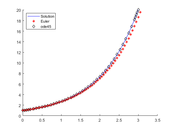
The method used in Matlab and Octave is a fair bit different from the methods discussed previously. We don’t need to go too much in detail about it, but some information will be helpful. The main difference that will be visible when running these methods is that they are adaptive method. This means that they adjust the step-size based on what the differential equation looks like at a given point. Euler’s method, along with the improved Euler and Runge-Kutta methods, is a fixed step-size method, where the steps are always the same no matter what. Adaptive methods are harder to write and optimize, but can solve many problems faster because the adaptive nature of the method allows them to get similar accuracy to fixed step methods, but at many fewer steps. In the example below, the initial value problem
\begin{equation*}
\frac{dy}{dt} = y \qquad y(0) = 1
\end{equation*}
is solved with an Euler’s method and Matlab’s built-in ode45 method. Both of the solutions are plotted along with the actual solution \(y = e^t\)
The Euler’s method takes 60 steps in this computation, but is still not as accurate as the ode45 method, which only takes 45 steps. In addition, the black diamonds, representing the different values computed by ode45 are not evenly spaced, illustrating the adaptive nature of this solver, while the red stars are all evenly spaced in the \(t\)-direction, as is expected from Euler’s method.
Consider the differential equation \(\frac{dy}{dt} = t^2 - 3y + 1\) with \(y(1)
= 4\text{.}\) Approximate the solution at \(t=3\) using Euler’s method with a step size of \(h=1\) and \(h=0.5\text{.}\) Compare these values with the actual solution at \(t=3\text{.}\)
Consider the differential equation \(\frac{dy}{dt} = 2ty + y^2\) with \(y(0)
= 1\text{.}\) Approximate the solution at \(t=2\) using Euler’s method with a step size of \(h=1\) and \(h=0.5\text{.}\)
Let \(x' = \sin(xt)\text{,}\) and \(x(0)=1\text{.}\) Approximate \(x(1)\) using Euler’s method with step sizes 1, 0.5, 0.25. Use a calculator and compute up to 4 decimal digits.
Approximate the value of \(e\) by looking at the initial value problem \(y'=y\) with \(y(0)=1\) and approximating \(y(1)\) using Euler’s method with a step size of \(0.2\text{.}\)
Example of numerical instability: Take \(y' = -5y\text{,}\)\(y(0) = 1\text{.}\) We know that the solution should decay to zero as \(x\) grows. Using Euler’s method, start with \(h=1\) and compute \(y_1, y_2, y_3, y_4\) to try to approximate \(y(4)\text{.}\) What happened? Now halve the interval. Keep halving the interval and approximating \(y(4)\) until the numbers you are getting start to stabilize (that is, until they start going towards zero). Note: You might want to use a calculator.
For \(h=1\text{,}\)\(y_4 = 256\text{.}\)\(h=0.5\text{,}\)\(y_4 = 25.6289\text{,}\)\(h=0.25\) goes to zero, but oscillates. \(h=0.125\) just goes to zero.
There is a simple way to improve Euler’s method to make it a second order method by doing just one extra step. Consider \(\frac{dy}{dx}=f(x,y)\text{,}\)\(y(x_0) =
y_0\text{,}\) and a step size \(h\text{.}\) What we do is to pretend we compute the next step as in Euler, that is, we start with \((x_i,y_i)\text{,}\) we compute a slope \(k_1
= f(x_i,y_i)\text{,}\) and then look at the point \((x_i+h,y_i + k_1h)\text{.}\) Instead of letting our new point be \((x_i+h,y_i + k_1h)\text{,}\) we compute the slope at that point, call it \(k_2\text{,}\) and then take the average of \(k_1\) and \(k_2\text{,}\) hoping that the average is going to be closer to the actual slope on the interval from \(x_i\) to \(x_i+h\text{.}\) And we are correct, if we halve the step, the error should go down by a factor of \(2^2 = 4\text{.}\) To summarize, the setup is the same as for regular Euler, except the computation of \(y_{i+1}\) and \(x_{i+1}\text{.}\)
The simplest method used in practice is the Runge-Kutta Method. Consider \(\frac{dy}{dx}=f(x,y)\text{,}\)\(y(x_0) = y_0\text{,}\) and a step size \(h\text{.}\) Everything is the same as in Euler’s method, except the computation of \(y_{i+1}\) and \(x_{i+1}\text{.}\)