For nonlinear systems, trajectories do not simply need to approach or leave a single point. They may in fact approach a larger set, such as a circle or another closed curve.
\begin{equation*}
x''-\mu(1-x^2) x' + x = 0,
\end{equation*}
where \(\mu\) is some positive constant. The Van der Pol oscillator originated with electrical circuits, but finds applications in diverse fields such as biology, seismology, and other physical sciences.
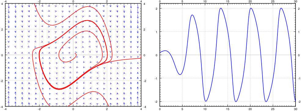
For simplicity, let us use \(\mu = 1\text{.}\) A phase diagram is given in the left-hand plot in Figure 5.4.2. Notice how the trajectories seem to very quickly settle on a closed curve. On the right-hand side is the plot of a single solution for \(t=0\) to \(t=30\) with initial conditions \(x(0) = 0.1\) and \(x'(0) = 0.1\text{.}\) The solution quickly tends to a periodic solution.
The Van der Pol oscillator is an example of so-called relaxation oscillation. The word relaxation comes from the sudden jump (the very steep part of the solution). For larger \(\mu\) the steep part becomes even more pronounced, for small \(\mu\) the limit cycle looks more like a circle. In fact, setting \(\mu = 0\text{,}\) we get \(x''+x=0\text{,}\) which is a linear system with a center and all trajectories become circles.
For example, the closed curve in the phase portrait for the Van der Pol equation is a limit cycle, and the limit cycle in the Van der Pol oscillator is asymptotically stable.
Given a closed trajectory on an autonomous system, any solution that starts on it is periodic. Such a curve is called a periodic orbit. More precisely, if \(\bigl(x(t),y(t)\bigr)\) is a solution such that for some \(t_0\) the point \(\bigl(x(t_0),y(t_0)\bigr)\) lies on a periodic orbit, then both \(x(t)\) and \(y(t)\) are periodic functions (with the same period). That is, there is some number \(P\) such that \(x(t) = x(t+P)\) and \(y(t) = y(t+P)\text{.}\)
We would like to be able to identify when these sorts of periodic orbits can or can’t happen to understand more about these systems. Thankfully, we have a theorem that gives us some help here.
Suppose \(R\) is a closed bounded region (a region in the plane that includes its boundary and does not have points arbitrarily far from the origin). Suppose \(\bigl(x(t), y(t)\bigr)\) is a solution of (5.4.1) in \(R\) that exists for all \(t \geq t_0\text{.}\) Then either the solution is a periodic function, or the solution tends towards a periodic solution in \(R\text{.}\)
is that if you find one solution that exists for all \(t\) large enough (that is, as \(t\) goes to infinity) and stays within a bounded region, then you have found either a periodic orbit, or a solution that spirals towards a limit cycle or tends to a critical point. That is, in the long term, the behavior is very close to a periodic function. Note that a constant solution at a critical point is periodic (with any period). The theorem is more a qualitative statement rather than something to help us in computations. In practice it is hard to find analytic solutions and so hard to show rigorously that they exist for all time. But if we think the solution exists we numerically solve for a large time to approximate the limit cycle. Another caveat is that the theorem only works in two dimensions. In three dimensions and higher, there is simply too much room.
The theorem applies to all solutions in the Van der Pol oscillator. Solutions that start at any point except the origin \((0,0)\) will tend to the periodic solution around the limit cycle, and if the initial condition of \((0,0)\) will lead to the constant solution \(x=0\text{,}\)\(y=0\text{.}\)
\begin{equation*}
x' = y + {(x^2+y^2-1)}^2 x, \qquad
y' = -x + {(x^2+y^2-1)}^2 y.
\end{equation*}
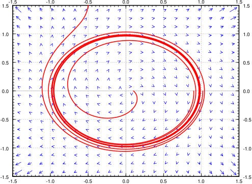
A vector field along with solutions with initial conditions \((1.02,0)\text{,}\)\((0.9,0)\text{,}\) and \((0.1,0)\) are drawn in Figure 5.4.6. Analyze this system to determine what will happen to the solution for a variety of initial conditions.
Notice that points on the unit circle (distance one from the origin) satisfy \(x^2+y^2-1=0\text{.}\) And \(x(t) = \sin(t)\text{,}\)\(y = \cos(t)\) is a solution of the system. Therefore we have a closed trajectory. For points off the unit circle, the second term in \(x'\) pushes the solution further away from the \(y\)-axis than the system \(x' = y\text{,}\)\(y' = -x\text{,}\) and \(y'\) pushes the solution further away from the \(x\)-axis than the linear system \(x'=y\text{,}\)\(y' = -x\text{.}\) In other words for all other initial conditions the trajectory will spiral out.
This means that for initial conditions inside the unit circle, the solution spirals out towards the periodic solution on the unit circle, and for initial conditions outside the unit circle the solutions spiral off towards infinity. Therefore the unit circle is a limit cycle, but not an asymptotically stable one. In relation to the terms used for autonomous equations in Section 1.7, we could refer to this as a semistable limit cycle, since on one side (inside) the solutions spiral towards the periodic orbit, while on the other side (outside) the solutions move away. The Poincaré-Bendixson Theorem applies to the initial points inside the unit circle, as those solutions stay bounded, but not to those outside, as those solutions go off to infinity.
\begin{equation*}
x' = y + {(x^2+y^2-1)} x, \qquad
y' = -x + {(x^2+y^2-1)} y.
\end{equation*}
We still obtain a closed trajectory on the unit circle, and points outside the unit circle spiral out to infinity, but now points inside the unit circle spiral towards the critical point at the origin. So this system does not have a limit cycle, even though it has a closed trajectory.
One way to see this more explicitly is by trying to write this all in terms of
\begin{equation*}
r = \sqrt{x^2 + y^2}.
\end{equation*}
For simplicity here, we will determine everything in terms of
\begin{equation*}
s = r^2 = x^2 + y^2
\end{equation*}
because as long as \(r > 0\text{,}\)\(r\) and \(s\) always have the same behavior (in terms of increasing and decreasing), and it is easier to compute with \(s\text{.}\)
which is an autonomous first-order equation that we can analyze. We have two equilibrium solutions in terms of \(s\) at \(s=0\text{,}\) which corresponds to the origin, and \(s=1\text{,}\) which corresponds to the unit circle. We can then plug in values to see that for \(s = \frac{1}{2}\text{,}\)\(\frac{ds}{dt} > 0\text{,}\) so that the solutions will increase out to the unit circle. For \(s>1\text{,}\)\(\frac{ds}{dt} > 0\) as well, so solutions move away from the circle outside it. This is the same as the result we obtained in the first example.
which is negative for \(0 < s < 1\) and positive for \(1 < s\text{,}\) giving that solutions that start inside the unit circle will converge to the origin, and solutions that start outside the circle will move away from it.
Due to the Picard theorem (Theorem 4.1.14) we find that no matter where we are in the plane we can always find a solution a little bit further in time, as long as \(f\) and \(g\) have continuous derivatives. So if we find a closed trajectory in an autonomous system, then for every initial point inside the closed trajectory, the solution will exist for all time and it will stay bounded (it will stay inside the closed trajectory). Since the closed trajectory is a solution, we can not cross it (by Picard theorem), and so we have to stay trapped inside. So the moment we found the solution above going around the unit circle, we knew that for every initial point inside the circle, the solution exists for all time and the Poincaré-Bendixson theorem applies.
Let us next look for conditions when limit cycles (or periodic orbits) do not exist. We assume the equation (5.4.1) is defined on a simply connected region, that is, a region with no holes we can go around. For example the entire plane is a simply connected region, and so is the inside of the unit disc. However, the entire plane minus a point is not a simply connected domain as it has a “hole” at the origin.
Suppose \(R\) is a simply connected region, and the expression 3
Usually the expression in the Bendixson-Dulac Theorem is \(\frac{\partial (\varphi f)}{\partial x} + \frac{\partial (\varphi
g)}{\partial y}\) for some continuously differentiable function \(\varphi\text{.}\) For simplicity, let us just consider the case \(\varphi = 1\text{.}\)
is either always positive or always negative on \(R\) (except perhaps a small set such as on isolated points or curves) then the system (5.4.1) has no closed trajectory inside \(R\text{.}\)
Henri Dulac (1870-1955) was a French mathematician.
gives us a way of ruling out the existence of a closed trajectory, and hence a way of ruling out limit cycles. The exception about points or curves means that we can allow the expression to be zero at a few points, or perhaps on a curve, but not on any larger set.
The entire plane is simply connected and so we can apply the theorem. We compute \(\frac{\partial f}{\partial x} + \frac{\partial g}{\partial y} =
y^2e^x+ 0\text{.}\) The function \(y^2e^x\) is always positive except on the line \(y=0\text{.}\) Therefore, via the theorem, the system has no closed trajectories.
In some books (or the internet) the theorem is not stated carefully and it concludes there are no periodic solutions. That is not quite right. The example above has two critical points and hence it has constant solutions, and constant functions are periodic. The conclusion of the theorem should be that there exist no trajectories that form closed curves. Another way to state the conclusion of the theorem would be to say that there exist no nonconstant periodic solutions that stay in \(R\text{.}\)
We compute \(\frac{\partial f}{\partial x} + \frac{\partial g}{\partial y} =
-2x + 2y=2(-x+y)\text{.}\) This expression takes on both signs, so if we are talking about the whole plane we cannot simply apply the theorem. However, we could apply it on the set where \(-x+y \geq 0\text{.}\) Via the theorem, there is no closed trajectory in that set. Similarly, there is no closed trajectory in the set \(-x+y \leq 0\text{.}\) We cannot conclude (yet) that there is no closed trajectory in the entire plane. Perhaps half of it is in the set where \(-x+y \geq 0\) and the other half is in the set where \(-x+y \leq 0\text{.}\)
The key is to look at the line where \(-x+y=0\text{,}\) or \(x=y\text{.}\) On this line \(x' = -y-x^2 = -x-x^2\) and \(y' = -x+y^2 = -x+x^2\text{.}\) In particular, when \(x=y\) then \(x' \leq y'\text{.}\) That means that the arrows, the vectors \((x',y')\text{,}\) always point into the set where \(-x+y \geq 0\text{.}\) There is no way we can start in the set where \(-x+y \geq 0\) and go into the set where \(-x+y \leq 0\text{.}\) Once we are in the set where \(-x+y \geq 0\text{,}\) we stay there. So no closed trajectory can have points in both sets.
Consider \(x' = y+(x^2+y^2-1)x\text{,}\)\(y' = -x +(x^2+y^2-1)y\text{,}\) and consider the region \(R\) given by \(x^2+y^2 >
\frac{1}{2}\text{.}\) That is, \(R\) is the region outside a circle of radius \(\frac{1}{\sqrt{2}}\) centered at the origin. Then there is a closed trajectory in \(R\text{,}\) namely \(x=\cos(t)\text{,}\)\(y=\sin(t)\text{.}\) Furthermore,
which is always positive on \(R\text{.}\) So what is going on? The Bendixson-Dulac theorem does not apply since the region \(R\) is not simply connected—it has a hole, the circle we cut out!
\(r=0\) is asymptotically stable, \(r=1\) is a periodic solution, but not a limit cycle, is unstable, \(r=4\) is semistable, limit cycle from the inside.
Does the system (5.4.2) have a limit cycle? If so, find it. If not, explain why not. For each positive root of \(f(r)\text{,}\) decide whether the corresponding trajectory one is stable, unstable, or semistable.
Suppose an autonomous system in the plane has a solution \(x=\cos(t)+e^{-t}\text{,}\)\(y=\sin(t)+e^{-t}\text{.}\) What can you say about the system (in particular about limit cycles and periodic solutions)?
Using Poincaré-Bendixson Theorem, the system has a limit cycle, which is the unit circle centered at the origin as \(x=\cos(t)+e^{-t}\text{,}\)\(y=\sin(t)+e^{-t}\) gets closer and closer to the unit circle. Thus we also have that \(x=\cos(t)\text{,}\)\(y=\sin(t)\) is the periodic solution.
Formulate a condition for a 2-by-2 linear system \({\vec{x}}' = A \vec{x}\) to not be a center using the Bendixson-Dulac theorem. That is, the theorem says something about certain elements of \(A\text{.}\)
A system such as \(x'=x, y'=y\) has solutions that exist for all time \(t\text{,}\) yet there are no closed trajectories. Explain why the Poincaré-Bendixson Theorem does not apply.
Show that the limit cycle of the Van der Pol oscillator (for \(\mu > 0\)) must not lie completely in the set where \(-1 < x < 1\text{.}\) Compare with Figure 5.4.2.
\(f(x,y) = y\text{,}\)\(g(x,y) = \mu(1-x^2)y-x\text{.}\) So \(f_x+g_y = \mu(1-x^2)\text{.}\) The Bendixson-Dulac Theorem says there is no closed trajectory lying entirely in the set \(x^2 < 1\text{.}\)
Differential equations can also be given in different coordinate systems. Suppose we have the system \(r' = 1-r^2\text{,}\)\(\theta' = 1\) given in polar coordinates. Find all the closed trajectories and check if they are limit cycles and if so, if they are asymptotically stable or not.
The closed trajectories are those where \(\sin(r) = 0\text{,}\) therefore, all the circles centered at the origin with radius that is a multiple of \(\pi\) are closed trajectories.