Existence and Uniqueness of Solutions

Section 1.5 Existence and Uniqueness of Solutions

Objectives

After this section, you will be able to:

🔗

Understand the terms existence and uniqueness as they apply to differential equations and
🔗

🔗
Find the maximum guaranteed interval of existence for the solution to an initial value problem.
🔗

🔗

🔗

If we take the differential equation

\begin{equation*} y' = f(x,y) \qquad y(x_0) = y_0, \end{equation*}

there are two main questions we want to answer about this equation.

🔗

Does a solution exist to the differential equation?
🔗

🔗
Is there only one solution to the differential equation?
🔗

🔗

🔗

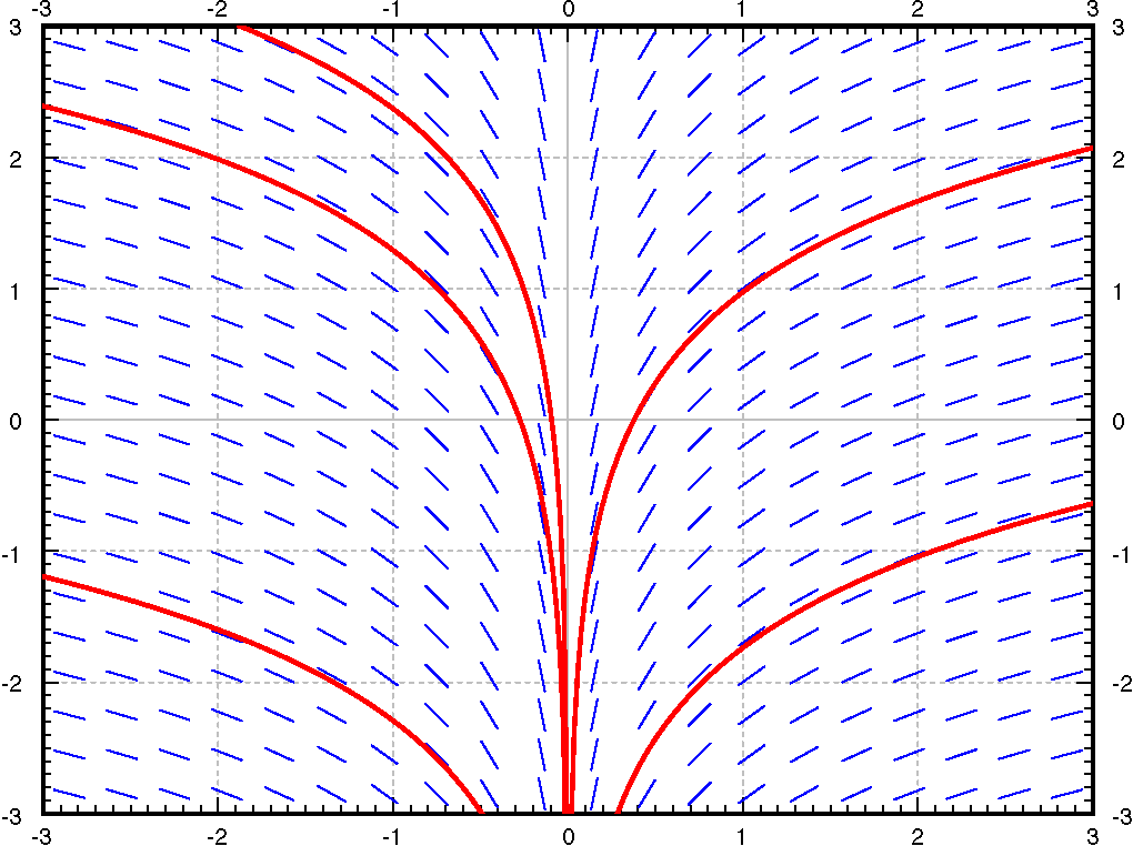
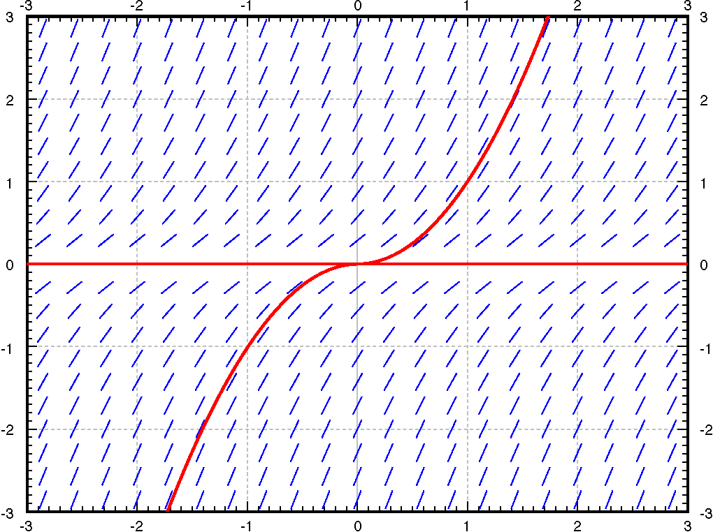
These are more commonly referred to as (a) existence of the solution and (b) uniqueness of the solution. These are especially crucial for equations that we are using to model a physical situation. For physical situations, the solution definitely exists (because the system does something and continues to exist) and the solution is unique, because a given system will always do the same thing given the same setup. Since we know that physical systems obey these properties, the equations we use to model them should have these properties as well. These properties do not necessarily hold for all differential equations, as shown in the examples below.

🔗

Example 1.5.1. Non-Existence of Solution.

Attempt to solve:

\begin{equation*} y' = \frac{1}{x}, \qquad y(0) = 0 . \end{equation*}

🔗

Answer.

Integrate to find the general solution $y = \ln \, \lvert x \rvert + C\text{.}$ The solution does not exist at $x=0\text{.}$ See Figure 1.5.2. The equation may have been written as the seemingly harmless $x y' = 1\text{.}$

🔗

ALT TEXT HERE — Figure 1.5.2. Slope field for $y' = \frac{1}{x}\text{.}$
🔗

🔗

Example 1.5.3. Non-Uniqueness of Solution.

Solve:

\begin{equation*} y' = 2 \sqrt{\lvert y \rvert}, \qquad y(0) = 0 . \end{equation*}

🔗

Answer.

See Figure 1.5.4. Note that $y=0$ is a solution. But another solution is the function

\begin{equation*} y(x) = \begin{cases} x^2 & \text{if } \; x \geq 0,\\ -x^2 & \text{if } \; x < 0. \end{cases} \end{equation*}

🔗

What we see here is a significant problem for trying to represent physical situations. In the first there is no solution at $x=0\text{,}$ so if our physical scenario had wanted one, that would be an issue. Similarly, for the second, we do have solutions, but we have two of them, so we can’t use this to predict what is going to happen to a physical situation modeled by this equation over time. So, we need both existence and uniqueness to hold for our modeling equation in order to use differential equations to accurately model situations. Thankfully, these properties do apply to most equations, and we have fairly straight-forward criteria that can be used to determine if these properties are true for a given differential equation. For a first-order linear differential equation, the theorem is fairly straight-forward.

🔗

Theorem 1.5.5.

Assume that we have the first-order linear differential equation given by

\begin{equation*} y' + p(x)y = g(x). \end{equation*}

If $p(x)$ and $g(x)$ are continuous functions on an interval $I$ that contains a point $x_0\text{,}$ then for any $y$-value $y_0\text{,}$ the initial value problem

\begin{equation*} y' + p(x)y = g(x) \qquad y(x_0) = y_0 \end{equation*}

has a unique solution. This solution exists and is unique on the entire interval $I\text{.}$

🔗

The idea and proof of this theorem comes from the fact that we have an explicit method for solving these equations no matter what $p$ and $g$ are. We can always find an integrating factor for the equation, convert the left-hand side into a product rule term, take a definite integral of both sides, and then solve for $y\text{.}$ Since we have this explicit formula, the solution will exist and be defined on the entire interval where the functions $p$ and $g$ are continuous. This also means that we can answer questions about where and for what values of $x$ the solution to a differential equation exists.

🔗

Example 1.5.6. Existence and Uniqueness for Linear Equations.

Consider the differential equation

\begin{equation*} (x-1)y' + \frac{1}{x-5} y = e^x \end{equation*}

What do the existence and uniqueness theorems say about the solution to this differential equation with the initial condition $y(2) = 6\text{?}$ What about the solution with initial condition $y(-3) = 1\text{?}$

🔗

Solution.

To apply the existence and uniqueness theorem, we need to get the $y'$ term by itself. This results in the differential equation

\begin{equation*} y' + \frac{1}{(x-1)(x-5)} y = \frac{e^x}{x-1}. \end{equation*}

In order to figure out where this solution exists and is unique, we need to determine where the coefficient functions $p(x)$ and $g(x)$ are continuous. The only two points that we have discontinuities are at $x=1$ and $x=5\text{.}$ Therefore, if we have the initial condition $y(2) = 6\text{,}$ we start at the $x$ value of $2\text{.}$ Because this equation is linear, it will exist everywhere that these two functions are both continuous containing the point $x=2\text{,}$ and since the only discontinuities are at $1$ and $5\text{,}$ we know that they are both continuous on $(1,5)\text{.}$ This means that we can take $(1,5)$ as the interval $I$ in the theorem, and know that this solution will exist and be unique on the interval $(1,5)\text{.}$

🔗

For the other initial condition, $y(-3) = 1\text{,}$ we now want an interval where these functions are continuous that contains $-3\text{.}$ Again, we only have to avoid $x=1$ and $x=5\text{,}$ so we can take the interval $(-\infty, 1)$ as the interval $I$ in the theorem, and so we know the solution with this initial condition will exist and be unique on $(-\infty, 1)\text{.}$

🔗

A convenient way to represent this situation is with a number line like that presented in Figure 1.5.7. On this number line, we mark the places where the functions $p(x)$ or $g(x)$ are discontinuous.

🔗

To interpret this image, we can mark the initial point on the number line, where the point that we mark is the x coordinate of the initial condition. All of the intervals are in terms of $x\text{.}$ Then, the existence and uniqueness theorem says that the solution will exist on the entire interval between any marked points on this number line. From that, we can see that the interval of existence for the initial condition $y(2) = 6$ is $(1,5)\text{,}$ and the interval for $y(-3) = 1$ is $(-\infty, 1)\text{.}$

🔗

For non-linear equations, we don’t have an explicit method of getting a solution that works for all equations. This means that we can’t fall back on this formula to guarantee existence or uniqueness of solutions. For this reason, we expect to get a result that is not as strong for non-linear equations. Thankfully, we do still get a result, which is known as Picard’s theorem

Named after the French mathematician Charles Émile Picard (1856-1941)

🔗

Theorem 1.5.8. Picard’s theorem on existence and uniqueness.

If $f(x,y)$ is continuous (as a function of two variables) and $\frac{\partial f}{\partial y}$ exists and is continuous near some $(x_0,y_0)\text{,}$ then a solution to

\begin{equation*} y' = f(x,y), \qquad y(x_0) = y_0, \end{equation*}

exists (at least for some small interval of $x$’s) and is unique.

🔗

The main fact that is “not as strong” about this result is the interval that we get from the theorem. For the linear theorem, we got existence and uniqueness on the entire interval $I$ where $p$ and $g$ are continuous. For the non-linear theorem, we only get existence on some interval around the point $x_0\text{.}$ Even if $f(x,y)$ and $\frac{\partial f}{\partial y}$ are really nice functions that are continuous everywhere, we can still only guarantee existence on a small interval (that can depend on the initial condition) around the point $x_0\text{.}$

🔗

Example 1.5.9. Interval of Existence for Non-Linear Equation.

For some constant $A\text{,}$ solve:

\begin{equation*} y' = y^2, \qquad y(0) = A . \end{equation*}

🔗

Solution.

We know how to solve this equation. First assume that $A \not= 0\text{,}$ so $y$ is not equal to zero at least for some $x$ near 0. So $x' = \nicefrac{1}{y^2}\text{,}$ so $x = \nicefrac{-1}{y} + C\text{,}$ so $y = \frac{1}{C-x}\text{.}$ If $y(0) = A\text{,}$ then $C = \nicefrac{1}{A}$ so

\begin{equation*} y = \frac{1}{\nicefrac{1}{A} - x} . \end{equation*}

If $A=0\text{,}$ then $y=0$ is a solution.

🔗

For example, when $A=1$ the solution is

\begin{equation*} y = \frac{1}{1-x} \end{equation*}

which goes to infinity, and so “blows up”, at $x=1\text{.}$ This solution here exists only on the interval $(-\infty, 1)\text{,}$ and hence, the solution does not exist for all $x$ even if the equation is nice everywhere. The equation $y' = y^2$ certainly looks nice.

🔗

However, this fact does not contradict our existence and uniqueness theorem for non-linear equations. The theorem only guarantees that the solution to

\begin{equation*} y' = y^2 \end{equation*}

exists and is unique on some interval containing 0. It does not guarantee that the solution exists everywhere that $y^2$ and its derivative are continuous, only that at each point where this happens, the solution will exist for some interval around that point. The interval $(-\infty, 1)$ is “some interval containing zero”, so the theorem still applies and holds here. See the exercises for more detail on how this process works and how we can illustrate the fact that the interval of existence is “some interval containing zero”.

🔗

The other main conclusion that we can draw from these theorems is the fact that two different solution curves to a first-order differential equation can not cross, provided the existence and uniqueness theorems hold. If $y_1$ and $y_2$ are two different solutions to $y' = f(x,y)$ and the solution curves for $y_1(x)$ and $y_2(x)$ cross, then this means that for some particular value of $x_0$ and $y_0\text{,}$ we have that

\begin{equation*} y_1(x_0) = y_0 \qquad y_2(x_0) = y_0. \end{equation*}

If we pick $x_0$ as a starting point, then the fact that the existence and uniqueness theorems hold imply that, at least for some interval around $x_0\text{,}$ there is exactly one solution to

\begin{equation*} y' = f(x,y) \qquad y(x_0) = y_0. \end{equation*}

However, both $y_1$ and $y_2$ satisfy these two properties. Therefore, $y_1$ and $y_2$ must be the same, which doesn’t make sense because we assumed they were different. So it is impossible for two different solution curves to cross, provided the existence and uniqueness theorem holds. For a comparison, refer back to Example 1.5.3 earlier to see what non-uniqueness looks like, where we do have two solution curves that cross at the point $(0,0)\text{.}$

🔗

This fact is useful for analyzing differential equations in general, but will be particularly useful in Section 1.7 in dealing with autonomous equations, where we can use simple solutions to provide boundaries over which other solutions can not cross. This fact will come up again in Chapter 4 and Chapter 5 in sketching trajectories for these solutions as well.

🔗

Example 1.5.10. Application of Uniqueness.

Consider the differential equation

\begin{equation*} \frac{dy}{dt} = (y-3)^2(y+4). \end{equation*}

🔗

Verify that $y=3$ is a solution to this differential equation.
🔗

🔗
Assume that we solve this problem with initial condition $y(0) = 1\text{.}$ Is it possible for this solution to ever reach $y=4\text{?}$ Why or why not?
🔗

🔗

🔗

Solution.

If we take the function $y(t) = 3\text{,}$ then $y' = 0\text{,}$ and plugging this into the right hand side also gives $0\text{.}$ Therefore, this function solves the differential equation.
🔗

🔗
If the solutions starts with $y(0) = 1\text{,}$ this means that it starts below the line $y=3\text{.}$ In order to get up to $y=4\text{,}$ the solution would need to cross over the line $y=3\text{,}$ which would mean that we have solution curves that cross. However, the function $f(t,y) = (y-3)^2(y+4)$ is continuous everywhere, as is the first derivative $\frac{\partial f}{\partial y} = 2(y-3)(y+4) + (y-3)^2.$ Therefore, the existence and uniqueness theorem applies everywhere, and so solution curves can not cross. So, it is not possible for the solution to reach $y=4\text{,}$ because this would force solution curves to cross, which we know can not happen.
🔗

🔗

🔗

Exercises Exercises

1.

Is it possible to solve the equation $y' = \frac{xy}{\cos x}$ for $y(0) = 1\text{?}$ Justify.

🔗

Answer.

Yes.

🔗

2.

Is it possible to solve the equation $y' = y\sqrt{\lvert x\rvert}$ for $y(0) = 0\text{?}$ Is the solution unique? Justify.

🔗

Answer.

Yes

🔗

3.

Consider the differential equation $y' + \frac{1}{t-2}y = \frac{1}{t+3}\text{.}$

🔗

(a)

Is this equation linear or non-linear?

🔗

Answer.

Linear

🔗

(b)

What is the maximum guaranteed interval of existence for the solution to this equation with initial condition $y(0) = 3\text{?}$

🔗

Answer.

$(-3,2)$

🔗

(c)

What if we start with the initial condition $y(4) = 0\text{?}$

🔗

Answer.

$(2,\infty)$

🔗

4.

Consider the differential equation $y' + \frac{1}{t+2}y = \frac{\ln(|t|)}{t-4}\text{.}$

🔗

(a)

Is this equation linear or non-linear?

🔗

Answer.

Linear

🔗

(b)

What is the maximum guaranteed interval of existence for the solution to this equation with initial condition $y(-3) = 1\text{?}$

🔗

Answer.

$(-\infty, -2)$

🔗

(c)

What if we start with the initial condition $y(2) = 5\text{?}$

🔗

Answer.

$(0, 4)$

🔗

(d)

What happens if we want to start with $y(4) = 3\text{?}$

🔗

Answer.

Nothing is guaranteed.

🔗

5.

Consider the differential equation $(t+3)y' + t^2 y = \frac{1}{t-2}\text{.}$

🔗

(a)

Is this equation linear or non-linear?

🔗

Answer.

Linear

🔗

(b)

What is the maximum guaranteed interval of existence for the solution to this equation with initial condition $y(-2) = 1\text{?}$

🔗

Answer.

$(-3, 2)$

🔗

(c)

What if we start with the initial condition $y(-4) = 5\text{?}$

🔗

Answer.

$(-\infty, -3)$

🔗

(d)

What happens if we want to start with $y(4) = 2\text{?}$

🔗

Answer.

$(2,\infty)$

🔗

6.

Consider the differential equation $y' = y^2\text{.}$

🔗

(a)

Is this equation linear or non-linear?

🔗

Answer.

Non-linear

🔗

(b)

What is the most we can say about the interval of existence for the solution to this equation with initial condition $y(0) = 1\text{?}$

🔗

Answer.

It will exist on some interval around $t=0\text{.}$

🔗

(c)

Find the solution to this differential equation with $y(0) = 1\text{.}$ Over what values of $x$ does this solution exist?

🔗

Answer.

$y = \frac{-1}{t-1}\text{,}$ $(-\infty, 1)$

🔗

(d)

Find the solution to this differential equation with $y(0) = 4\text{.}$ Over what values of $x$ does this solution exist?

🔗

Answer.

$y = \frac{-1}{t - \frac{1}{4}}\text{,}$ $\left(-\infty, \frac{1}{4}\right)$

🔗

(e)

Find the solution to this differential equation with $y(0) = -2\text{.}$ Over what values of $x$ does this solution exist?

🔗

Answer.

$y = \frac{-1}{t+2}\text{,}$ $(-2, \infty)$

🔗

(f)

Do any of these contradict your answer in (b)?

🔗

Answer.

No. All of these are intervals containing zero.

🔗

7.

Consider the differential equation $y' = y^2 + 4\text{.}$

🔗

(a)

Is this equation linear or non-linear?

🔗

Answer.

Non-linear

🔗

(b)

What is the most we can say about the interval of existence for the solution to this equation with initial condition $y(0) = 0\text{?}$

🔗

Answer.

Some interval around zero.

🔗

(c)

Find the solution to this differential equation with $y(0) = 0\text{.}$ Over what values of $x$ does this solution exist?

🔗

Answer.

$y = 2\tan(2t)\text{,}$ Exists on $\left(-\frac{\pi}{4}, \frac{\pi}{4}\right)$

🔗

8.

Consider the differential equation $y' = x(y+1)^2\text{.}$

🔗

(a)

Is this equation linear or non-linear?

🔗

Answer.

Non-linear

🔗

(b)

If we set $f(x,y) = x(y+1)^2\text{,}$ for what values of $x$ and $y$ are $f$ and $\frac{\partial f}{\partial y}$ continuous? What is the most we can say about the interval of existence for the solution to this equation with initial condition $y(0) = 1\text{?}$

🔗

Answer.

Some interval around $t=0$

🔗

(c)

Find the solution to this differential equation with $y(0) = 1\text{.}$ Over what values of $x$ does this solution exist?

🔗

Answer.

$y = \frac{2}{1-x^2} - 1\text{,}$ Exists on $(-1, 1)$

🔗

9.

Take $(y-x)y' = 0\text{,}$ $y(0) = 0\text{.}$

🔗

(a)

Find two distinct solutions.

🔗

Answer.

$y=0$ and $y=x$

🔗

(b)

Explain why this does not violate Picard’s theorem.

🔗

Answer.

$f(x,y)$ is discontinuous when $x=y\text{,}$ and $(0,0)$ is one such point.

🔗

10.

Find a solution to $y' = \lvert y \rvert\text{,}$ $y(0) = 0\text{.}$ Does Picard’s theorem apply?

🔗

Answer.

$y=0$ or $y = \text{sign}(x)\frac{x^2}{2}\text{.}$ No.

🔗

11.

Consider the IVP $y'\cos t+y\sin t=1; \, y(\pi/6)=1\text{.}$

🔗

(a)

The Existence and Uniqueness Theorem guarantees a unique solution to this IVP on what interval?

🔗

Answer.

$\left(-\frac{\pi}{2}, \frac{\pi}{2}\right)$

🔗

(b)

Find this solution explicitly.

🔗

Answer.

$y = \sin(t) + \frac{1}{\sqrt{3}}\cos(t)$

🔗

12.

Take an equation $y' = (y-2x) g(x,y) + 2$ for some function $g(x,y)\text{.}$ Can you solve the problem for the initial condition $y(0) = 0\text{,}$ and if so what is the solution?

🔗

Answer.

$y = 2x$

🔗

13.

Consider the differential equation $y' = e^x(2-y)\text{.}$

🔗

(a)

Verify that $y = 2$ is a solution to this differential equation.

🔗

Answer.

Yes

🔗

(b)

Assume that we look for the solution with $y(0) = 0\text{.}$ Is it possible that $y(x) = 3$ for some later time $x\text{?}$ Why or why not?

🔗

Answer.

No.

🔗

(c)

Based on this, what do we know about the solution with $y(0) = 5\text{?}$

🔗

Answer.

Must stay above $2$ for all $x\text{.}$ Approaches 2.

🔗

14.

Suppose $y' = f(x,y)$ is such that $f(x,1) = 0$ for every $x\text{,}$ $f$ is continuous and $\frac{\partial f}{\partial y}$ exists and is continuous for every $x$ and $y\text{.}$

🔗

(a)

Guess a solution given the initial condition $y(0) = 1\text{.}$

🔗

Answer.

$y=1$

🔗

(b)

Can graphs of two solutions of the equation for different initial conditions ever intersect?

🔗

Answer.

🔗

(c)

Given $y(0) = 0\text{,}$ what can you say about the solution. In particular, can $y(x) > 1$ for any $x\text{?}$ Can $y(x) = 1$ for any $x\text{?}$ Why or why not?

🔗

Answer.

Must stay below $y=1$

🔗

15.

Consider the differential equation $y' = y^2 - 4\text{.}$

🔗

(a)

Verify that $y=2$ and $y=-2$ are both solutions to this differential equation.

🔗

Answer.

Yes

🔗

(b)

Verify that the hypotheses of Picard’s theorem are satisfies for this equation.

🔗

Answer.

Yes

🔗

(c)

Assume that we solve this differential equation with $y(0) = 1\text{.}$ Is it possible for the solution to reach $y=3$ at any point? Why or why not?

🔗

Answer.

🔗

(d)

Assume that we solve this differential equation with $y(0) = -1\text{.}$ Is it possible for the solution to reach $y=-4$ at any point? Why or why not?

🔗

Answer.

🔗

16.

Is it possible to solve $y' = xy$ for $y(0) = 0\text{?}$ Is the solution unique?

🔗

Answer.

Yes. Since $f$ and $\frac{\partial f}{\partial y}$ are both continuouns, this solution will be unique.

🔗

17.

Is it possible to solve $y' = \frac{x}{x^2-1}$ for $y(1) = 0\text{?}$

🔗

Answer.

No. $f$ is not continuous at this initial condition.

🔗

18.

Suppose

\begin{equation*} f(y) = \begin{cases} 0 & \text{ if $y > 0$}, \\ 1 & \text{ if $y \leq 0$} . \end{cases} \end{equation*}

Does $y' = f(y)\text{,}$ $y(0) = 0$ have a continuously differentiable solution? Does Picard apply? Why, or why not?

🔗

Answer.

Picard does not apply as $f$ is not continuous at $y=0\text{.}$ The equation does not have a continuously differentiable solution. Suppose it did. Notice that $y'(0) = 1\text{.}$ By the first derivative test, $y(x) > 0$ for small positive $x\text{.}$ But then for those $x$ we would have $y'(x) = 0\text{,}$ so clearly the derivative cannot be continuous.

🔗

19.

Consider an equation of the form $y' = f(x)$ for some continuous function $f\text{,}$ and an initial condition $y(x_0) = y_0\text{.}$ Does a solution exist for all $x\text{?}$ Why or why not?

🔗

Answer.

The solution is $y(x) = \int_{x_0}^x f(s) \,ds + y_0\text{,}$ and this does indeed exist for every $x\text{.}$

🔗

Prev Top Next