There is one remaining case for the two-component first-order linear system: repeated eigenvalues. As we have seen previously, it may happen that a matrix \(A\) has some “repeated” eigenvalues. That is, the characteristic equation \(\det(A-\lambda I) = 0\) may have repeated roots. This is actually unlikely to happen for a random matrix. If we take a small perturbation of \(A\) (we change the entries of \(A\) slightly), we get a matrix with distinct eigenvalues. As any system we want to solve in practice is an approximation to reality anyway, it is not absolutely indispensable to know how to solve these corner cases. On the other hand, these cases do come up in applications from time to time. Furthermore, if we have distinct but very close eigenvalues, the behavior is similar to that of repeated eigenvalues, and so understanding that case will give us insight into what is going on.
\(A\) has an eigenvalue 3 of multiplicity 2. We call the multiplicity of the eigenvalue in the characteristic equation the algebraic multiplicity. In this case, there also exist 2 linearly independent eigenvectors, \(\left[ \begin{smallmatrix} 1 \\ 0 \end{smallmatrix} \right]\) and \(\left[ \begin{smallmatrix} 0 \\ 1 \end{smallmatrix} \right]\) corresponding to the eigenvalue 3. This means that the so-called geometric multiplicity of this eigenvalue is also 2. These terms have all been discussed previously in Section 3.5.
In all the theorems where we required a matrix to have \(n\) distinct eigenvalues, we only really needed to have \(n\) linearly independent eigenvectors. For example, \({\vec{x}}' = A\vec{x}\) has the general solution
Let us restate the theorem about real eigenvalues. In the following theorem we will repeat eigenvalues according to (algebraic) multiplicity. So for the matrix \(A\) above, we would say that it has eigenvalues 3 and 3.
Suppose the \(n \times n\) matrix \(P\) has \(n\) real eigenvalues (not necessarily distinct), \(\lambda_1\text{,}\)\(\lambda_2\text{,}\) …, \(\lambda_n\text{,}\) and there are \(n\) linearly independent corresponding eigenvectors \(\vec{v}_1\text{,}\)\(\vec{v}_2\text{,}\) …, \(\vec{v}_n\text{.}\) Then the general solution to \({\vec{x}}' = P\vec{x}\) can be written as
The main difference in the statement here from the theorem in Section 4.4 is that we are no longer assuming that we have \(n\)distinct eigenvalues. Instead, we need to assume that we end up with \(n\) linearly independent eigenvectors, which we get for free if the eigenvalues are all distinct, but we might also have that if we do not have all distinct eigenvalues.
The geometric multiplicity of an eigenvalue of algebraic multiplicity \(n\) is equal to the number of corresponding linearly independent eigenvectors. The geometric multiplicity is always less than or equal to the algebraic multiplicity. The theorem handles the case when these two multiplicities are equal for all eigenvalues. If for an eigenvalue the geometric multiplicity is equal to the algebraic multiplicity, then we say the eigenvalue is complete.
In other words, the hypothesis of the theorem could be stated as saying that if all the eigenvalues of \(P\) are complete, then there are \(n\) linearly independent eigenvectors and thus we have the given general solution.
If the geometric multiplicity of an eigenvalue is 2 or greater, then the set of linearly independent eigenvectors is not unique up to multiples as it was before. For example, for the diagonal matrix \(A =
\left[ \begin{smallmatrix} 3 & 0 \\ 0 & 3 \end{smallmatrix} \right]\) we could also pick eigenvectors \(\left[ \begin{smallmatrix} 1 \\ 1 \end{smallmatrix} \right]\) and \(\left[ \begin{smallmatrix} 1 \\ -1 \end{smallmatrix} \right]\text{,}\) or in fact any pair of two linearly independent vectors. The number of linearly independent eigenvectors corresponding to \(\lambda\) is the number of free variables we obtain when solving \(A\vec{v} =
\lambda \vec{v}\text{.}\) We pick specific values for those free variables to obtain eigenvectors. If you pick different values, you may get different eigenvectors.
If an \(n \times n\) matrix has less than \(n\) linearly independent eigenvectors, it is said to be deficient. Then there is at least one eigenvalue with an algebraic multiplicity that is higher than its geometric multiplicity. We call this eigenvalue defective and the difference between the two multiplicities we call the defect.
We must have that \(v_2 = 0\text{.}\) Hence any eigenvector is of the form \(\left[ \begin{smallmatrix} v_1 \\ 0 \end{smallmatrix} \right]\text{.}\) Any two such vectors are linearly dependent, and hence the geometric multiplicity of the eigenvalue is 1. Therefore, the defect is 1, and we can no longer apply the eigenvalue method directly to a system of ODEs with such a coefficient matrix.
Roughly, the key observation is that if \(\lambda\) is an eigenvalue of \(A\) of algebraic multiplicity \(m\text{,}\) then we can find certain \(m\) linearly independent vectors solving \({(A-\lambda I)}^k \vec{v} = \vec{0}\) for various powers \(k\text{.}\) We will call these generalized eigenvectors.
Let us continue with the example \(A = \left[ \begin{smallmatrix}
3 & 1 \\ 0 & 3
\end{smallmatrix} \right]\) and the equation \({\vec{x}}' = A\vec{x}\text{.}\) We found an eigenvalue \(\lambda=3\) of (algebraic) multiplicity 2 and defect 1. We found one eigenvector \(\vec{v} = \left[ \begin{smallmatrix} 1 \\ 0 \end{smallmatrix} \right]\text{.}\) We have one solution
We are now stuck, we get no other solutions from standard eigenvectors. But we need two linearly independent solutions to find the general solution of the equation.
Since there is no \(e^{3t}\) term on the right-hand side of the equation, we are forced to pick \(\vec{v}_1 = \vec{0}\text{,}\) and so we get the solution \(\vec{x}_2 = \vec{0}\text{,}\) which is not good. This guess did not work.
The issue here is that we didn’t have enough flexibility to actually get another solution to the differential equation, so we need something a little more complicated to make it work. To this end, we take a new guess of the form
As we are assuming that \(\vec{x}_2\) is a solution, \({\vec{x}_2}'\) must equal \(A \vec{x}_2\text{.}\) So let’s compute \(A \vec{x}_2\text{:}\)
\begin{equation*}
A \vec{x}_2 =
A ( \vec{v}_2 + \vec{v}_1 t )\, e^{3t}
=
A \vec{v}_2 e^{3t} + A \vec{v}_1 t e^{3t} .
\end{equation*}
By looking at the coefficients of \(e^{3t}\) and \(t e^{3t}\) we see \(3 \vec{v}_2 + \vec{v}_1 = A \vec{v}_2\) and \(3 \vec{v}_1 = A \vec{v}_1\text{.}\) This means that
Therefore, \(\vec{x}_2\) is a solution if these two equations are satisfied. The second equation is satisfied if \(\vec{v}_1\) is an eigenvector, and we found the eigenvector above, so let \(\vec{v}_1 =
\left[ \begin{smallmatrix} 1 \\ 0 \end{smallmatrix} \right]\text{.}\) So, if we can find a \(\vec{v}_2\) that solves \((A-3I)\vec{v}_2 = \vec{v}_1\text{,}\) then we are done. This is just a bunch of linear equations to solve and we are by now very good at that. Let us solve \((A-3I)\vec{v}_2 = \vec{v}_1\text{.}\) Write
By inspection we see that letting \(a=0\) (\(a\) could be anything in fact) and \(b=1\) does the job. Hence we can take \(\vec{v}_2 =
\left[ \begin{smallmatrix} 0 \\ 1 \end{smallmatrix} \right]\text{.}\) Our general solution to \({\vec{x}}' = A\vec{x}\) is
Let us check that we really do have the solution. First \(x_1' =
c_1 3 e^{3t}+c_2 e^{3t} + 3 c_2 te^{3t} = 3 x_1 + x_2\text{.}\) Good. Now \(x_2' = 3 c_2 e^{3t} = 3x_2\text{.}\) Good.
Furthermore, if \((A-3I) \vec{w} \not= \vec{0}\text{,}\) then \((A-3I) \vec{w}\) is an eigenvector, a multiple of \(\vec{v}_1\text{.}\) In this \(2 \times 2\) case \({(A-3I)}^2\) is just the zero matrix (exercise). So any vector \(\vec{w}\) solves \({(A-3I)}^2\vec{w} = \vec{0}\) and we just need a \(\vec{w}\) such that \((A-3I)\vec{w} \not= \vec{0}\text{.}\) Then we could use \(\vec{w}\) for \(\vec{v}_2\text{,}\) and \((A-3I)\vec{w}\) for \(\vec{v}_1\text{.}\)
Note that the system \({\vec{x}}' = A \vec{x}\) has a simpler solution since \(A\) is a so-called upper triangular matrix, that is every entry below the diagonal is zero. In particular, the equation for \(x_2\) does not depend on \(x_1\text{.}\) Mind you, not every defective matrix is triangular.
Solve \({\vec{x}}' = \left[ \begin{smallmatrix}
3 & 1 \\ 0 & 3
\end{smallmatrix} \right] \vec{x}\) by first solving for \(x_2\) and then for \(x_1\) independently. Check that you got the same solution as we did above.
Let us describe the general algorithm. Suppose that \(\lambda\) is an eigenvalue of multiplicity 2, defect 1. First find an eigenvector \(\vec{v}_1\) of \(\lambda\text{.}\) That is, \(\vec{v}_1\) solves \((A-\lambda I)\vec{v}_1 = \vec{0}\text{.}\) Then, find a vector \(\vec{v}_2\) such that
These two equations are redundant, and the first equation is \(-3v_1 + 3v_2 = 0\text{,}\) which can be solved by \(v_1 = v_2 = 1\text{.}\) Therefore, and an eigenvector for \(\lambda = 1\) is \(\left[ \begin{smallmatrix} 1 \\ 1 \end{smallmatrix} \right]\text{.}\) Thus, we have a solution to this system of the form
and both rows of the vector equation result in the equation \(-3w_1 + 3w_2 = 1\) for \(\vec{w}\text{.}\) We can pick any value of \(w_1\) and \(w_2\) to make this work. For the sake of this example, we will pick \(w_1 = 0\) and \(w_2 = \nicefrac{1}{3}\text{.}\) Then, we have that our second linearly independent solution to the differential equation is
which gives that \(c_1 = 2\) and then \(2 + \nicefrac{1}{3}c_2 = -1\text{,}\) or \(c_2 = -9\text{.}\) Therefore, the solution to the initial value problem is
We could have also chosen \(w_1 = -\nicefrac{1}{3}\) and \(w_2 = 0\) for the vector \(\vec{w}\text{.}\) Use this to get a different looking general solution. Then solve the same initial value problem to see that you end up with the same answer at the end of the process.
Even though this is a three-component system, the process is exactly the same: find the eigenvalues, compute corresponding eigenvectors, then build them together into a general solution. Compute the eigenvalues,
The eigenvalues are 1 and 2, where 2 has multiplicity 2. We leave it to the reader to find that \(\left[ \begin{smallmatrix} 0 \\ 0 \\ 1 \end{smallmatrix} \right]\) is an eigenvector for the eigenvalue \(\lambda = 1\text{.}\)
The first equation says that \(v_2 = 0\text{,}\) so the last equation is \(-v_1 -v_3 = 0\text{.}\) Let \(v_3\) be the free variable to find that \(v_1 = -v_3\text{.}\) Perhaps let \(v_3 = -1\) to find an eigenvector \(\left[ \begin{smallmatrix} 1 \\ 0 \\ -1 \end{smallmatrix} \right]\text{.}\) Problem is that setting \(v_3\) to anything else just gets multiples of this vector and so we have a defect of 1. Let \(\vec{v}_1\) be the eigenvector and let’s look for a generalized eigenvector \(\vec{v}_2\text{:}\)
\begin{equation*}
(A - 2 I) \vec{v}_2 = \vec{v}_1 ,
\end{equation*}
where we used \(a\text{,}\)\(b\text{,}\)\(c\) as components of \(\vec{v}_2\) for simplicity. The first equation says \(-5b = 1\) so \(b = \nicefrac{-1}{5}\text{.}\) The second equation says nothing. The last equation is \(-a + 4b - c = -1\text{,}\) or \(a + \nicefrac{4}{5} + c = 1\text{,}\) or \(a + c = \nicefrac{1}{5}\text{.}\) We let \(c\) be the free variable and we choose \(c=0\text{.}\) We find \(\vec{v}_2 = \left[ \begin{smallmatrix} \nicefrac{1}{5} \\ \nicefrac{-1}{5}
\\ 0 \end{smallmatrix} \right]\text{.}\)
This machinery can also be generalized to higher multiplicities and higher defects. We will not go over this method in detail, but let us just sketch the ideas. Suppose that \(A\) has an eigenvalue \(\lambda\) of multiplicity \(m\text{.}\) We find vectors such that
Such vectors are called generalized eigenvectors (then \(\vec{v}_1 = {(A - \lambda I)}^{k-1} \vec{v}_k\) is an eigenvector). For the eigenvector \(\vec{v}_1\) there is a chain of generalized eigenvectors \(\vec{v}_2\) through \(\vec{v}_k\) such that:
Really once you find the \(\vec{v}_k\) such that \({(A - \lambda I)}^k \vec{v}_k = \vec{0}\) but \({(A - \lambda I)}^{k-1} \vec{v}_k \not= \vec{0}\text{,}\) you find the entire chain since you can compute the rest, \(\vec{v}_{k-1} = (A - \lambda I) \vec{v}_k\text{,}\)\(\vec{v}_{k-2} = (A - \lambda I) \vec{v}_{k-1}\text{,}\) etc. We form the linearly independent solutions
Recall that \(k! = 1 \cdot 2 \cdot 3 \cdots (k-1) \cdot k\) is the factorial. If you have an eigenvalue of geometric multiplicity \(\ell\text{,}\) you will have to find \(\ell\) such chains (some of them might be short: just the single eigenvector equation). We go until we form \(m\) linearly independent solutions where \(m\) is the algebraic multiplicity. We don’t quite know which specific eigenvectors go with which chain, so start by finding \(\vec{v}_k\) first for the longest possible chain and go from there.
For example, if \(\lambda\) is an eigenvalue of \(A\) of algebraic multiplicity 3 and defect 2, then solve
\begin{equation*}
(A - \lambda I) \vec{v}_1 = \vec{0} , \qquad
(A - \lambda I) \vec{v}_2 = \vec{v}_1 , \qquad
(A - \lambda I) \vec{v}_3 = \vec{v}_2 .
\end{equation*}
That is, find \(\vec{v}_3\) such that \({(A - \lambda I)}^3 \vec{v}_3 = \vec{0}\text{,}\) but \({(A - \lambda I)}^2 \vec{v}_3 \not= \vec{0}\text{.}\) Then you are done as \(\vec{v}_2 = (A - \lambda I) \vec{v}_3\) and \(\vec{v}_1 = (A - \lambda I) \vec{v}_2\text{.}\) The 3 linearly independent solutions are
If on the other hand \(A\) has an eigenvalue \(\lambda\) of algebraic multiplicity 3 and defect 1, then solve
\begin{equation*}
(A - \lambda I) \vec{v}_1 = \vec{0} , \qquad
(A - \lambda I) \vec{v}_2 = \vec{0} , \qquad
(A - \lambda I) \vec{v}_3 = \vec{v}_2 .
\end{equation*}
Here \(\vec{v}_1\) and \(\vec{v}_2\) are actual honest eigenvectors, and \(\vec{v}_3\) is a generalized eigenvector. So there are two chains. To solve, first find a \(\vec{v}_3\) such that \({(A - \lambda I)}^2 \vec{v}_3 = \vec{0}\text{,}\) but \((A - \lambda I) \vec{v}_3 \not= \vec{0}\text{.}\) Then \(\vec{v}_2 = (A - \lambda I) \vec{v}_3\) is going to be an eigenvector. Then solve for an eigenvector \(\vec{v}_1\) that is linearly independent from \(\vec{v}_2\text{.}\) You get 3 linearly independent solutions
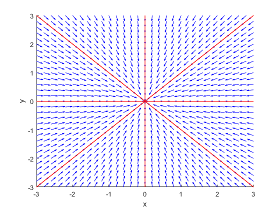
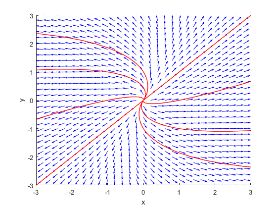
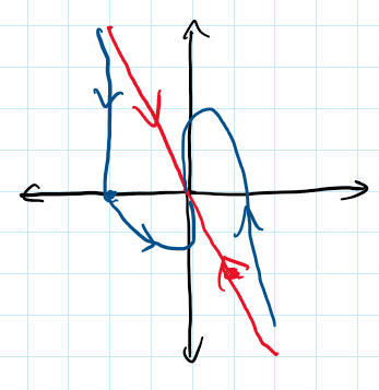
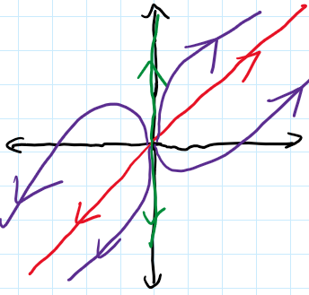
We also want to look at the phase portraits and direction field diagrams for repeated eigenvalues. There are two different options here, depending on if there are two linearly independent eigenvectors or not.
for the repeated eigenvalue \(\lambda\text{.}\) This means that \(A \vec{v} = \lambda \vec{v}\) for all vectors \(\vec{v}\text{.}\) So, every vector is part of a straight line solution, and so every solution goes either directly towards or directly away from the origin. This gives a proper node which can be a sink or a source depending on whether the eigenvalue is positive or negative.
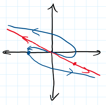
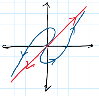
Case 2. If we have a repeated eigenvalue with only one linearly independent eigenvector, then we only have one straight-line solution. For instance, the matrix
has only one eigenvector of \(\begin{bmatrix} 1 \\ 1 \end{bmatrix}\) for eigenvalue \(3\text{.}\) Like the nodal sources and sinks, the solutions will go to zero and infinity along the straight line solutions. In this case, because there is only one straight line, the phase portrait looks somewhere between a node and a spiral. This gives an improper node which can be a source or sink depending on the sign of the eigenvalue.
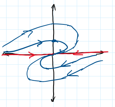
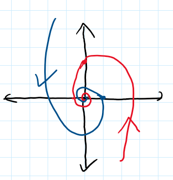
We also need to think about the direction of rotation for these improper nodes as well, as they somewhat act both like spirals and nodes. There are two ways of analyzing these phase portrait graphs again, and they follow the same tricks as their spiral counterparts.
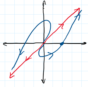
The \(C_1\) term gives our straight-line solution, so we need to consider the \(C_2\) term. We can rewrite this term as \(e^{3t}\left(\left[\begin{smallmatrix} 1 \\ 1 \end{smallmatrix}\right]t + \left[\begin{smallmatrix} 1 \\ 0 \end{smallmatrix}\right] \right)\text{.}\) At \(t=0\text{,}\) this term is at \(\left[\begin{smallmatrix} 1 \\ 0 \end{smallmatrix}\right]\text{,}\) and as \(t \rightarrow \infty\text{,}\) the solution ends up in the direction of \(\left[\begin{smallmatrix} 1 \\ 1 \end{smallmatrix}\right]\text{,}\) so it is in the first quadrant. Therefore, our solution starts at the point \((1,0)\) and ends up in the first quadrant as \(t \rightarrow \infty\text{.}\) Since this is an improper source, this means the solution is also going away from the origin as \(t \rightarrow \infty\text{.}\) Therefore, the solution goes off to \(\infty\) in the first quadrant (along the straight line solution) as \(t\rightarrow \infty\text{,}\) and going backwards, it has to flip around to the opposite side of the straight-line solution. This gives the sketch that we see in Figure 4.6.8.
The second method again involves the bottom-left entry of the matrix. Again, this is positive, which means that our rotation is in the counter-clockwise direction. It is a little trickier to prove in this case (you need to use the structure of the generalized eigenvector), but it works out in the same way. This means that below the \(\left[\begin{smallmatrix} 1 \\ 1 \end{smallmatrix}\right]\) straight-line solution, the solution spirals counter-clockwise as \(t\) gets larger, which means that it has to leave the origin along the \(\left[\begin{smallmatrix} -1 \\ -1 \end{smallmatrix}\right]\) direction, rotate around counter-clockwise, and head away from the origin along the \(\left[\begin{smallmatrix} 1 \\ 1 \end{smallmatrix}\right]\) direction. That’s the only way it can rotate counter-clockwise.
In both of these cases, the curve on the other side of the straight-line solution must mirror it. This puts together the entire sketch of the phase portrait for these improper nodes. The other point to be especially careful about is that having an improper nodal source and improper nodal sink look opposite, even if they have the same direction of rotation. The direction always refers to \(t\) increasing, not going into or away from the origin.
Let \(A = \left[ \begin{smallmatrix} 5 & -3 \\ 3 & -1 \end{smallmatrix} \right]\text{.}\) Find the general solution of \({\vec{x}}' = A \vec{x}\) and sketch the corresponding phase portrait.
Suppose that \(A\) is a \(2 \times 2\) matrix with a repeated eigenvalue \(\lambda\text{.}\) Suppose that there are two linearly independent eigenvectors. Show that \(A = \lambda I\text{.}\)
Let \(A =
\left[ \begin{smallmatrix}
a & a \\
b & c
\end{smallmatrix}\right]\text{,}\) where \(a\text{,}\)\(b\text{,}\) and \(c\) are unknowns. Suppose that \(5\) is a doubled eigenvalue of defect 1, and suppose that \(\left[ \begin{smallmatrix}
1 \\ 0
\end{smallmatrix}\right]\) is a corresponding eigenvector. Find \(A\) and show that there is only one such matrix \(A\text{.}\)
Convert this equation into a first order linear system using the transformation \(\vec{x} = \left[ \begin{smallmatrix} y \\ y' \end{smallmatrix} \right]\text{.}\)
Convert this equation into a first order linear system using the transformation \(\vec{x} = \left[ \begin{smallmatrix} y \\ y' \end{smallmatrix} \right]\text{.}\)
Convert this equation into a first order linear system using the transformation \(\vec{x} = \left[ \begin{smallmatrix} y \\ y' \end{smallmatrix} \right]\text{.}\)