Section 1.10 Modeling with First Order Equations

One of the main reasons to study and learn about differential equations, particularly for scientists and engineers, is their application and use in mathematical modeling. Since the derivative of a function represents the rate of change of that quantity, if we can use physical or scientific principles to develop an equation for the rate of change of some quantity in terms of the quantity and time, there’s a chance that we can write a differential equation for this quantity and solve it to determine how the quantity will change.

Subsection Principles of Mathematical Modeling

The process of mathematical modeling involves three main steps. The first of these is to write the model. This part comes from basic science or engineering principles and involves writing a differential equation that fits the given situation. If we can determine the rate at which a quantity will change based on the surrounding factors, we have a good shot of getting to such an equation. One main principle that can be used to write these equations is the accumuilation equation, which will be discussed in the next subsection.
The second step of this process is to solve the differential equation. This can mean either an analytic solution or a numeric one, and this is where the work of this class comes into play. We are going through a bunch of different techniques for solving differential equations and analyzing the overall behavior of such equations so that we can use them in this way. The end goal is to get an equation or a graph for how the quantity that we made a model for is going to change in time.
The final step of the process is to validate the model by comparing with experimental data. Once we have written the model and solved the corresponding differential equation, we want to make sure that the model works. To do this, we can take a new version of the original scenario, run the model as well as the physical experiment and see how the results compare. If the results are β€œclose” (in whatever sense makes logical sense for the problem), then we have a good model and can keep it. However, if our results differ significantly, then the model we used probably doesn’t apply to this problem. We need to go back to step 1 to try to figure out a better model for the physical situation in order to get more accurate results.
Why do we care about mathematical modeling? The biggest thing that it does from an engineering point of view is reduce the need for repeated testing. If we have a mathematical model that works for a given physical system, we can see how the system will be have under slightly different conditions and with different initial conditions without needing to run the physical experiment over and over again. We can do all of this testing on the model, and since we have validated the model, we can assume that the actual results will be similar. This also allows us to change some aspects of the physical situation to try to optimize it, but do so just by modifying the mathematical model, not the physical setup. This can significantly cut down on costs and allow for more optimal system design at the same time.

Subsection The Accumulation Equation

The accumulation equation is one of the simplest general mathematical formulations that can be used to develop mathematical models. This equation comes down to the fact that the rate of change of some quantity should be equal to the rate at which it is being added minus the rate at which it is being removed. If we let \(x\) be the quantity in question, this can be written as
\begin{equation} \frac{dx}{dt} = \text{rate in} - \text{rate out}.\tag{1.10.1} \end{equation}
This may seem fairly simple. However, it shows up in many places in science and engineering. Any mass or energy balance equations are examples of accumulation equations. These types of equations can also be written for the accumulation of momentum, and doing so for fluids gives rise to the Navier-Stokes equations, providing the basis for several fields of engineering. The examples that we see here will be simpler than that, but the idea is still the same.

Example 1.10.1.

A tank initially contains 70 gallons of water and 5 lbs of salt. A solution with salt concentration 0.2 lbs per gallon flows into the tank at a rate of \(3\) gal/min. The tank is well stirred, and water is removed from the tank at a rate of \(3\) gal/min. Find the amount of salt in the tank at any time \(t\text{?}\) What happens as \(t\rightarrow \infty\text{?}\) Does this make sense?
Solution.
To solve this problem, we use the accumulation equation (1.10.1) on the amount of salt in the tank. In order to compute with this, we recognize that in terms of mass of salt moving into the tank
\begin{equation*} \text{rate in} = \text{flow in} \times \text{concentration in} \end{equation*}
and similarly for the mass of salt leaving the tank.
If we let \(x\) represent the amount of salt in the tank at any time \(t\) (which is the goal of the problem), we can write a differential equation for this using the accumulation equation (1.10.1). This gives us that
\begin{equation*} \frac{dx}{dt} = \text{rate in} - \text{rate out} = \text{flow in} \times \text{concentration in} - \text{flow out} \times \text{concentration out} \end{equation*}
For this problem, we have that
\begin{align*} \text{flow in} \amp = 3\\ \text{concentration in} \amp = 0.2 \\ \text{flow out} \amp = 3 \\ \text{concentration out}\amp = \frac{x}{\text{volume}} = \frac{x}{70} \text{.} \end{align*}
The last of these lines comes from the fact that the tank is β€œwell-stirred” or β€œwell-mixed.” This implies that the concentration of salt in the water leaving the tank is the same as the concentration in the tank, which we can compute as \(\frac{x}{\text{volume}}\text{.}\) In this case, since the flow rate in and out are both 3 gal/min, the volume of water in the tank is fixed at \(70\) gallons, so we can put this in the equation.
Therefore, our equation becomes
\begin{equation*} \frac{dx}{dt} = (3\times 0.2) - \left(3 \times \frac{x}{70}\right). \end{equation*}
We can rewrite this equation as
\begin{equation*} \frac{dx}{dt} + \frac{3}{70}x = 0.6 \end{equation*}
which we recognize as a first order linear equation. We can then solve this using the method of integrating factors. Our factor \(r(t)\) is
\begin{equation*} r(t) = e^{\int p(t)\, dt} = e^{\int \frac{3}{70}\, dt} = e^{\frac{3}{70} t}, \end{equation*}
which we can multiply on both sides of the equation to obtain
\begin{equation*} e^{\frac{3}{70} t} \frac{dx}{dt} + e^{\frac{3}{70} t} \frac{3}{70} x = 0.6 e^{\frac{3}{70} t}. \end{equation*}
The left side of this is a product rule derivative, so we can integrate both sides to obtain
\begin{equation*} e^{\frac{3}{70} t} x = 0.6 \frac{70}{3} e^{\frac{3}{70} t} + C. \end{equation*}
We can then isolate \(x\) to get our general solution as
\begin{equation*} x = 14 + Ce^{-\frac{3}{70} t}. \end{equation*}
Our initial condition tells us that \(x(0) = 5\text{.}\) Plugging this in gives that
\begin{equation*} 5 = x(0) = 14 + C \quad \Rightarrow \quad C = -9, \end{equation*}
so the solution to the initial value problem, and thus our calculation for the amount of salt in the tank at any time \(t\text{,}\) is
\begin{equation*} x(t) = 14 - 9e^{-\frac{3}{70} t}. \end{equation*}
As \(t\rightarrow \infty\text{,}\) we see that the exponential term goes to zero. This leaves us with 14 lbs of salt in the tank after a long time. This makes some sense because this would give us a concentration of \(\frac{14}{70} = 0.2\) lb/gal, and that was exactly the concentration of the in-flow stream. It makes sense that after a long time of mixing and removing water from the tank, the concentration of the tank would match that of the incoming stream.
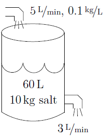
The same principle works for other types of examples, including those where the volume of the tank is not constant in time.
ALT TEXT HERE
IMAGE DESCRIPTION HERE
Figure 1.10.2. Sketch of the modeling problem for a tank where the volume of water increases with time.

Example 1.10.3.

A 100 liter tank contains 10 kilograms of salt dissolved in 60 liters of water. Solution of water and salt (brine) with concentration of 0.1 kilograms per liter is flowing in at the rate of 5 liters a minute. The solution in the tank is well stirred and flows out at a rate of 3 liters a minute. How much salt is in the tank when the tank is full?
Solution.
We can again use the accumulation equation to write
\begin{equation*} \frac{dx}{dt} = (\text{flow in} \times \text{concentration in}) - (\text{flow out} \times \text{concentration out}) . \end{equation*}
In this example, we have
\begin{align*} \text{flow in} \amp = 5 \\ \text{concentration in} \amp = 0.1 \\ \text{flow out} \amp = 3 \\ \text{concentration out} \amp = \frac{x}{\text{volume}} = \frac{x}{60+(5-3)t} \end{align*}
Our equation is, therefore,
\begin{equation*} \frac{dx}{dt} = (5 \times 0.1) - \left(3 \frac{x}{60+2t}\right) . \end{equation*}
Or in the form (1.4.1)
\begin{equation*} \frac{dx}{dt} + \frac{3}{60+2t} x = 0.5 . \end{equation*}
Let us solve. The integrating factor is
\begin{equation*} r(t) = \exp \left( \int \frac{3}{60+2t} dt \right) = \exp \left( \frac{3}{2} \ln (60+2t) \right) = {(60+2t)}^{3/2} . \end{equation*}
We multiply both sides of the equation by this \(r(t)\) to get
\begin{align*} {(60+2t)}^{3/2} \frac{dx}{dt} + {(60+2t)}^{3/2} \frac{3}{60+2t} x \amp = 0.5{(60+2t)}^{3/2} \\ \frac{d}{dt}\left[ {(60+2t)}^{3/2} x \right] \amp = 0.5{(60+2t)}^{3/2} \\ {(60+2t)}^{3/2} x \amp = \int 0.5{(60+2t)}^{3/2} dt +C \\ x \amp = {(60+2t)}^{-3/2} \int \frac{ {(60+2t)}^{3/2} }{2} dt +C{(60+2t)}^{-3/2} \\ x \amp = {(60+2t)}^{-3/2} \frac{1}{10}{(60+2t)}^{5/2} +C{(60+2t)}^{-3/2} \\ x \amp = \frac{60+2t}{10} +C{(60+2t)}^{-3/2} \text{.} \end{align*}
ALT TEXT HERE
IMAGE DESCRIPTION HERE
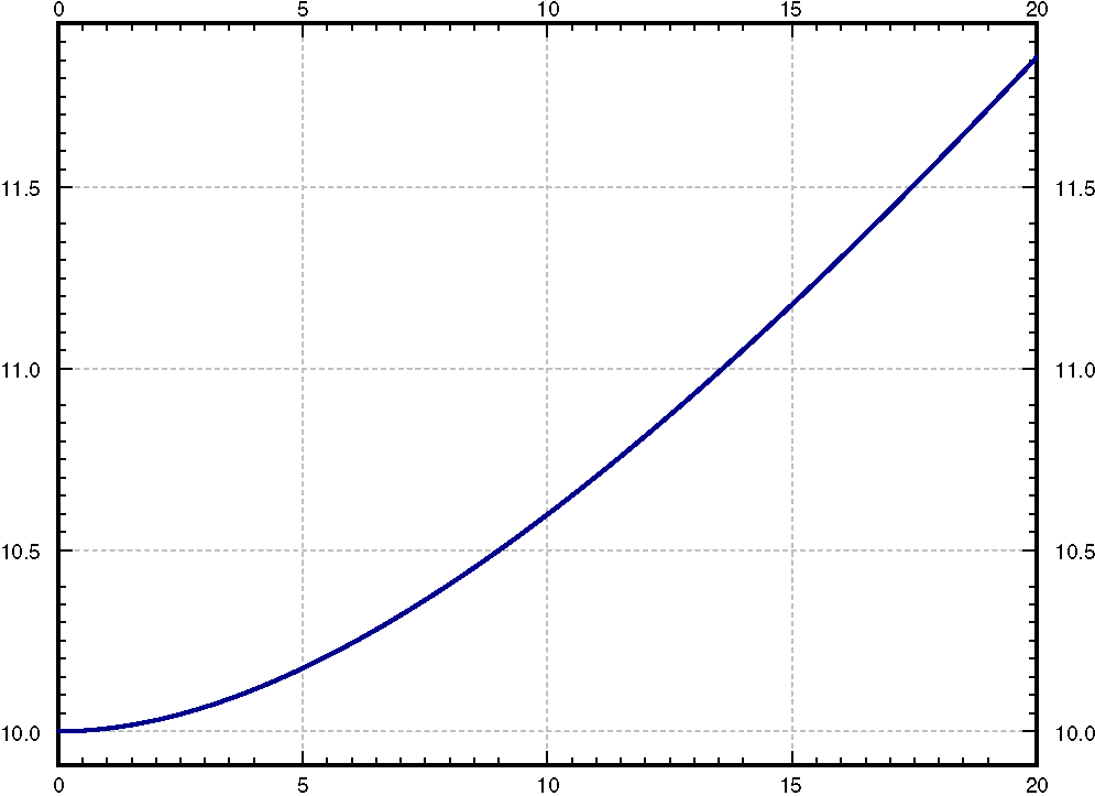
Figure 1.10.4. Graph of the solution \(x\) kilograms of salt in the tank at time \(t\text{.}\)
We need to find \(C\text{.}\) We know that at \(t=0\text{,}\) \(x=10\text{.}\) So
\begin{equation*} 10 = x(0) = \frac{60}{10} +C{(60)}^{-3/2} = 6 +C{(60)}^{-3/2} , \end{equation*}
or
\begin{equation*} C=4 ({60}^{3/2}) \approx 1859.03 . \end{equation*}
We are interested in \(x\) when the tank is full. The tank is full when \(60+2t = 100\text{,}\) or when \(t=20\text{.}\) So
\begin{align*} x(20) \amp = \frac{60+40}{10}+C{(60+40)}^{-3/2}\\ \amp \approx 10+1859.03 {(100)}^{-3/2} \approx 11.86 \text{.} \end{align*}
See FigureΒ 1.10.4 for the graph of \(x\) over \(t\text{.}\)
The concentration when the tank is full is approximately \(\unitfrac[0.1186]{kg}{liter}\text{,}\) and we started with \(\nicefrac{1}{6}\) or \(\unitfrac[0.167]{kg}{liter}\text{.}\)
For the previous example, we obtained the solution
\begin{equation*} x(t) = \frac{60 + 2t}{10} + 1859.03(60+2t)^{-3/2}, \end{equation*}
which is valid and well defined for all positive values of \(t\) (it has an issue at \(t=-30\text{,}\) but we aren’t concerned about that here). However, as a differential equation that represents a physical situation, it is not valid for all positive values of \(t\text{.}\) The issue here is that the tank is full at \(t=20\text{.}\) Therefore, beyond this point, while the function still exists, it is not a valid model for this physical system. Once the tank fills, you can’t keep adding and removing water at the same rates that you have been up until this point, because something is going to break with the system. The same goes for if you are removing water from the tank at a faster rate than you are adding it, because then the tank will empty at some point in time and beyond that, the model equation no longer represents the system.
The same ideas apply to problems involving interest compounded continuously. For an interest rate of \(r\text{,}\) the β€œrate in,” or the rate at which the money in the account is increasing, is \(rP\) where \(P\) is the amount of money in the account. Taking this along with other factors that may affect the balance of the account allows us to write a differential equation, which we can solve to determine what the balance will be over time.

Example 1.10.5. Compounded Interest.

A bank account with an interest rate of \(6\%\) per year, compounded continuously, starts with a balance of $30000. The owner of the account withdraws $50 from the account each month. Find and solve a differential equation for the account balance over time. What is the largest amount that the owner could withdraw each month without the account eventually reaching $0?
Solution.
We will use the function \(P(t)\) to model the balance of the account over time, where \(t\) is in years. Since the owner withdraws $50 per month, this means that they withdraw $600 over the course of the year. This means that the differential equation we want is
\begin{equation*} \frac{dP}{dt} = 0.06P - 600 \qquad P(0) = 30000. \end{equation*}
We can solve this equation by the integrating factor method.
\begin{align*} P' - 0.06P \amp= -600 \\ (e^{-0.06t}P)' \amp= -600e^{-0.06t} \\ e^{-0.06t}P \amp= 10000e^{-0.06t} + C \\ P \amp= 10000 + Ce^{0.06t} \text{.} \end{align*}
For \(P(0) = 30000\text{,}\) we need to take \(C = 20000\text{.}\) Thus, the solution to the initial value problem is
\begin{equation*} P(t) = 10000 + 20000e^{0.06 t}. \end{equation*}
Since the coefficient in front of \(e^{0.06t}\) is positive, this means that the account balance here will grow in time.
For the second part, we need to adjust the withdrawal amount to see how the solution changes. If we let \(K\) be the monthly withdrawal amount, then we have the differential equation
\begin{equation*} \frac{dP}{dt} = 0.06P - 12K \qquad P(0) = 30000. \end{equation*}
The same solution method gives us
\begin{equation*} P(t) = \frac{12K}{0.06} + Ce^{0.06t}. \end{equation*}
If \(C < 0\text{,}\) then the account balance will eventually go to zero. Therefore, we need \(C \geq 0\text{,}\) and since \(P(0) = 30000\text{,}\) we have that
\begin{equation*} 30000 = \frac{12K}{0.06} + C \quad \text{ or } \quad C = 30000 - \frac{12K}{0.06}. \end{equation*}
For this to be equal to zero, we need
\begin{equation*} \frac{12K}{0.06} = 30000 \qquad K = 150. \end{equation*}
Thus, the owner can withdraw $150 per month and keep the account balance positive.
To end this section, we will analyze the example that was presented at the very beginning of the book.

Example 1.10.6. Falling Object.

An object falling through the air has its velocity affected by two factors: gravity and a drag force. The velocity downward is increased at a rate of \(9.8\ m/s^2\) due to gravity, and it is decreased by a rate equation to \(0.3\) times the current velocity of the object. If the ball is initially thrown downwards at a speed of \(2\ m/s\text{,}\) what will the velocity be 10 seconds later?
Solution.
As described in that first section, we know that the differential equation that we can write for this situation is
\begin{equation*} \frac{dv}{dt} = 9.8 - 0.3v \end{equation*}
and that the initial condition for the velocity if \(v(0) = 2\text{.}\) Since we have gravity as a positive 9.8, this means that the downward direction is positive, so the object being thrown downward at \(2\ m/s\) means that it is positive. We then need to solve this initial value problem, which we can do using first order linear methods. The equation can be written as
\begin{equation*} v' + 0.3v = 9.8 \end{equation*}
which has integrating factor \(e^{0.3t}\text{.}\) After multiplying this to both sides and integrating, we get that
\begin{equation*} e^{0.3t}v = \frac{9.8}{0.3}e^{0.3t} + C \end{equation*}
or that
\begin{equation*} v(t) = \frac{9.8}{0.3} + Ce^{-0.3t}. \end{equation*}
Using the initial condition, we get that
\begin{equation*} v(0) = \frac{98}{3} + C = 2 \end{equation*}
so that \(C = -\frac{92}{3}\) and the solution to the initial value problem is
\begin{equation*} v(t) = \frac{98}{3} - \frac{92}{3}e^{-0.3t}. \end{equation*}
Then, to determine the velocity at \(t=10\text{,}\) we can plug \(10\) into this formula to get that
\begin{equation*} v(10) = \frac{98}{3} - \frac{92}{3}e^{-3} \approx 31.14\ m/s. \end{equation*}
All of these examples are based around the same idea of the accumulation equation. We need to determine the quantity that is changing as well as all of the factors that cause it to increase and decrease. These get combined into a differential equation which we can solve in order to analyze the situation and answer whatever questions you want about that physical problem. Keeping these ideas in mind will help you approach a wide variety of problems both in this class as well as future applications in engineering classes and beyond.

Exercises Exercises

1.

Suppose there are two lakes located on a stream. Clean water flows into the first lake, then the water from the first lake flows into the second lake, and then water from the second lake flows further downstream. The in and out flow from each lake is 500 liters per hour. The first lake contains 100 thousand liters of water and the second lake contains 200 thousand liters of water. A truck with 500 kg of toxic substance crashes into the first lake. Assume that the water is being continually mixed perfectly by the stream.
(a)
Find the concentration of toxic substance as a function of time in both lakes.
Answer.
\(c_1(t) = \frac{1}{200}e^{-t/200}\) \(c_2(t) = \frac{1}{200}(e^{-t/400} - e^{-t/200})\)

2.

Newton’s Law of Cooling states that \(\frac{dx}{dt} = -k(x-A)\) where \(x\) is the temperature, \(t\) is time, \(A\) is the ambient temperature, and \(k > 0\) is a constant. Suppose that \(A = A_0 \cos (\omega t)\) for some constants \(A_0\) and \(\omega\text{.}\) That is, the ambient temperature oscillates (for example night and day temperatures).
(a)
Find the general solution.
Answer.
\(x(t) = kA_0 \left(\frac{\omega \sin(\omega t) + k\cos(\omega t)}{\omega^2 + k^2}\right) + Ce^{-kt}\)
(b)
In the long term, will the initial conditions make much of a difference? Why or why not?
Answer.
No. Only in \(C\text{.}\)

3.

Initially 5 grams of salt are dissolved in 20 liters of water. Brine with concentration of salt 2 grams of salt per liter is added at a rate of 3 liters per minute. The tank is mixed well and is drained at 3 liters per minute. How long does the process have to continue until there are 20 grams of salt in the tank?
Answer.
\(\approx 3.73\) min

4.

Initially a tank contains 10 liters of pure water. Brine of unknown (but constant) concentration of salt is flowing in at 1 liter per minute. The water is mixed well and drained at 1 liter per minute. In 20 minutes there are 15 grams of salt in the tank. What is the concentration of salt in the incoming brine?
Answer.
\(\approx 1.735\) g/L

5.

Suppose a water tank is being pumped out at \(\unitfrac[3]{L}{min}\text{.}\) The water tank starts at \(\unit[10]{L}\) of clean water. Water with toxic substance is flowing into the tank at \(\unitfrac[2]{L}{min}\) , with concentration \(\unitfrac[$20t$]{g}{L}\) at time \(t\text{.}\) When the tank is half empty, how many grams of toxic substance are in the tank (assuming perfect mixing)?
Answer.
250 grams.

6.

A 300 gallon well-mixed water tank initially starts with 200 gallons of water and 15 lbs of salt. One stream with salt concentration one pound per gallon flows into the tank at a rate of 3 gallons per minute and water is removed from the well-mixed tank at a rate of 2 gallons per minute.
(a)
Write and solve an initial value problem for the volume of water in the tank at any time \(t\text{.}\)
Answer.
\(\frac{dV}{dt} = 1\text{,}\) \(V(0) = 200\text{.}\) \(V(t) = 200+t\text{.}\)
(b)
Set up an initial value problem for the amount of salt in the tank at any time \(t\text{.}\) You do not need to solve it (yet), but should make sure to state it fully.
Answer.
\(\frac{dQ}{dt} = 3 - \frac{2Q}{200+t}\text{,}\) \(Q(0) = 15\text{.}\)
(c)
Is the solution to this initial value problem a valid representation of the physical model for all times \(t > 0\text{?}\) If so, use the information in the equation to determine the long-time behavior of the solution. If not, explain why, determine the time when the representation breaks down, and what happens at that point in time.
Answer.
No. Overflows at \(t=100\text{.}\)
(d)
Solve the initial value problem above and compare this to your answer to the previous part.
Answer.
\(Q(t) = (200+t) - \frac{185(200)^2}{(200+t)^2}\) This function is defined for all positive \(t\text{.}\)

7.

A 500 gallon well-mixed water tank initially starts with 300 gallons of water and 200 lbs of salt. One stream with salt concentration of flows into the tank at a rate of and water is removed from the well-mixed tank at a rate of \(\unitfrac[7]{gal}{min}\text{.}\)
(a)
Write and solve an initial value problem for the volume of water in the tank at any time \(t\text{.}\)
Answer.
\(\frac{dV}{dt} = -2\text{,}\) \(V(0) = 300\text{.}\) \(V(t) = 300-2t\text{.}\)
(b)
Set up an initial value problem for the amount of salt in the tank at any time \(t\text{.}\) You do not need to solve it (yet), but should make sure to state it fully.
Answer.
\(\frac{dQ}{dt} = 2.5 - \frac{7Q}{300-2t}\text{,}\) \(Q(0) = 200\)
(c)
Is the solution to this initial value problem a valid representation of the physical model for all times \(t > 0\text{?}\) If so, use the information in the equation to determine the long-time behavior of the solution. If not, explain why, determine the time when the representation breaks down, and what happens at that point in time.
Answer.
No, tank empties at \(t = 150\text{.}\)
(d)
Solve the initial value problem above and compare this to your answer to the previous part.
Answer.
\(Q(t) = 0.5(300-2t) + \frac{50}{(300)^{7/2}}(300-2t)^{7/2}\text{.}\) \(Q(t)\) is negative for \(t > 150\text{.}\)

8.

A 200 gallon well-mixed water tank initially starts with 150 gallons of water and 50 lbs of salt. One stream with salt concentration of \(\unitfrac[0.2]{lb}{gal}\) flows into the tank at a rate of \(\unitfrac[4]{gal}{min}\) and water is removed from the well-mixed tank at a rate of \(\unitfrac[4]{gal}{min}\text{.}\)
(a)
Write and solve an initial value problem for the volume of water in the tank at any time \(t\text{.}\)
Answer.
\(\frac{dV}{dt} = 0\text{,}\) \(V(0) = 150\text{.}\) \(V(t) = 150\text{.}\)
(b)
Set up an initial value problem for the amount of salt in the tank at any time \(t\text{.}\) You do not need to solve it (yet), but should make sure to state it fully.
Answer.
\(\frac{dQ}{dt} = 0.8 - \frac{4}{150}Q\text{,}\) \(Q(0) = 50\text{.}\)
(c)
Is the solution to this initial value problem a valid representation of the physical model for all times \(t > 0\text{?}\) If so, use the information in the equation to determine the long-time behavior of the solution. If not, explain why, determine the time when the representation breaks down, and what happens at that point in time.
Answer.
Yes. Solution tends towards 30.
(d)
Solve the initial value problem above and compare this to your answer to the previous part.
Answer.
\(Q(t) = 30 + 20e^{-2t/75}\text{.}\) Matches.

9.

Suppose we have bacteria on a plate and suppose that we are slowly adding a toxic substance such that the rate of growth is slowing down. That is, suppose that \(\frac{dP}{dt} = (2-0.1\,t)P\text{.}\) If \(P(0) = 1000\text{,}\) find the population at \(t=5\text{.}\)
Answer.
\(P(5) = 1000 e^{2 \times 5 - 0.05 \times {5}^2} = 1000 e^{8.75} \approx 6.31 \times {10}^6\)

10.

A cylindrical water tank has water flowing in at \(I\) cubic meters per second. Let \(A\) be the area of the cross section of the tank in meters. Suppose water is flowing from the bottom of the tank at a rate proportional to the height of the water level. Set up the differential equation for \(h\text{,}\) the height of the water, introducing and naming constants that you need. You should also give the units for your constants.
Answer.
\(Ah' = I - kh\text{,}\) where \(k\) is a constant with units \(\unit{m^2}{s}\text{.}\)

11.

An object in free fall has a velocity that increases at a rate of 32 \(ft/s^2\text{.}\) Due to drag, the velocity decreases at a rate of 0.1 times the velocity of the object squared, when written in feet per second.
(b)
This equation is autonomous, so draw a phase diagram for this equation and classify all critical points.
Answer.
\(v = \sqrt{320}\) is asymptotically stable, \(v = -\sqrt{320}\) is unstable.
(c)
What will happen to the velocity if the object is dropped at \(t=0\text{?}\) What about if the object is thrown downwards at a rate of \(10 ft/s\text{?}\)
Answer.
Always tends towards \(\sqrt{320}\)

12.

The number of people in a town that support a given measure decays at a constant rate of \(10\) people per day. However, the support for the measure can be increased by individuals discussing the issue. This results in an increase of the support at a rate of \(ay(1000 - y)\) people per day, where \(y\) is the number of people who support the measure, and \(a\) is a constant depending on the way in which the issue is being discussed. Write a differential equation to model this situation, and determine the amount of people who will support the measure long-term if \(a\) is set to \(10^{-4}\text{.}\)
Answer.
\(\frac{dy}{dt} = ay(1000-y) - 10\text{,}\) \(=100(5 + \sqrt{15}) \approx 887.3\text{.}\)

13.

Newton’s Law of Procrastination states that the rate at which one accomplishes a chore is proportional to the amount of the chore not yet done. Unbeknownst to Newton, this applies to robots too. A Roomba is attempting to vacuum a house measuring 1000 square feet. When none of the house is clean, the roomba can clean 200 square feet per hour. What makes this problem fun is that there is also a dog. It’s whatever kind of dog you like, take your pick. The dog dirties the house at a constant rate of 50 square feet per hour.
(a)
Assume that none of the house is clean at \(t=0\text{.}\) Write a DE for the number of square feet that are clean as a function of time, and solve for that quantity.
Answer.
\(\frac{dy}{dt} = \frac{1}{5}(1000 - y) - 50 = 150 - \frac{1}{5}y\text{.}\) \(y(t) = 750(1-e^{-t/5})\)
(b)
How long will it take before the house is half clean? Will it ever be entirely clean? (Explain briefly.)
Answer.
\(t = 5\ln(3)\) for half clean. Never fully clean.

14.

A student has a loan for $50000 with 5% interest. The student makes $300 payments on the loan each month. The rate here is an annual rate, compounded continuously, and the differential equation you write should be in years.
(a)
With this setup, how long does it take the student to pay off the loan? How much money does the student pay over this period of time?
Answer.
\(27.712\) years or 285 months. Pays approximately $85,500
(b)
What is the minimal amount the student should pay each month if they want to pay off the loan within 5 years? How much does the student pay over this period?
Answer.
\(\approx \$942\)

15.

A factory pumps 6 tons of sludge per day into a nearby pond. The pond initially contains 100,000 gallons of water, and no sludge. Each day, 3,000 gallons of rain water falls into the pond, and 1,000 gallons per day leave the pond via a river. Assume, for no good reason, that the water leaving the pond has the same concentration of sludge as the pond as a whole. How much sludge will there be in the pond after 150 days?
Answer.
700 gallons

16.

In this exercise, we compare two different young people and their investment strategies. Both of these people are investing in an account with 7.5% annual rate of return. Person 1 invests $50 a month starting at age 20, and Person 2 invests $100 per month starting at age 30. Write differential equations to model each of these account balances over time, and compute the amount of money in each account at age 50. Who has more money in the account? Who has invested more money? What would person 2 have to invest each month in order for the two balances to be equal at age 50?
Answer.
Person 1 has more money (\(\approx \$67,902\) compared to \(\approx \$55,707\)). Person 2 has invested more (\(\$24,000\) compared to \(\$18,000\)). Person 2 needs to invest \(\approx \$122\text{.}\)

17.

Radioactive decay follows similar rules to interest, where a certain portion of the material decays over time, resulting in an equation of the form
\begin{equation*} \frac{dy}{dt} = -ky \end{equation*}
for some constant \(k\text{.}\) The half-life of a material is the amount of time that it takes for half of the material to have decayed away. Assume that the half-life of a given substance is \(T\) minutes. Find a formula for \(k\text{,}\) the coefficient in the decay equation, in terms of \(T\text{.}\)
Answer.
\(k = \frac{1}{T}\ln(2)\)