The next case to consider for constant coefficient second order equations is the one where \(b^2 - 4ac < 0\text{.}\) This results in two roots \(r_1\) and \(r_2\text{,}\) but they are complex roots. In order to solve differential equations with \(b^2 - 4ac < 0\text{,}\) we need to be able to manipulate and use some properties of complex numbers. Complex numbers may seem a strange concept, especially because of the terminology. There is nothing imaginary or really complicated about complex numbers. For more bachground information on complex numbers, see Section A.2.
To start with, we define \(i = \sqrt{-1}\text{.}\) Since this is the square root of a negative number, this \(i\) is not a real number. A complex number is written in the form \(z = x+iy\) where \(x\) and \(y\) are real numbers. For a complex number \(x+iy\) we call \(x\) the real part and \(y\) the imaginary part of the number. Often the following notation is used,
\begin{equation*}
\operatorname{Re}(x+iy) = x
\qquad \text{and} \qquad
\operatorname{Im}(x+iy) = y.
\end{equation*}
The real numbers are contained in the complex numbers as those complex numbers with the imaginary part being zero.
When trying to do arithmetic with complex numbers, we treat \(i\) as though it is a variable, and do computations just as we would with polynomials. The important fact that we will use to simplify is the fact that since \(i = \sqrt{-1}\text{,}\) we have that \(i^2 = -1\text{.}\) So whenever we see \(i^2\text{,}\) we replace it by \(-1\text{.}\) For example,
The numbers \(i\) and \(-i\) are the two roots of \(r^2 + 1 = 0\text{.}\) Engineers often use the letter \(j\) instead of \(i\) for the square root of \(-1\text{.}\) We use the mathematicians’ convention and use \(i\text{.}\)
The important part to keep in mind with complex numbers is that dividing by complex numbers is not as simple as one would hope. The process does not just involve inverting the real and imaginary parts and putting an \(i\) in there, instead, the complex number in the denominator needs to be converted into a real number by multiplying the top and bottom by the complex conjugate, and then everything can be distributed and simplified. We use \(\bar{z}\) to denote the complex conjugate of a complex number \(z\text{,}\) and for \(z = a+bi\) the conjugate is defined as \(\bar{z} = a - bi\text{.}\) Thus, if we multiply a complex number \(z = a+bi\) by its complex conjugate,
In order to solve differential equations where the characteristic equation has complex roots, we need to deal with the exponential \(e^{a+bi}\) of complex numbers. We do this by writing down the Taylor series and plugging in the complex number. Because most properties of the exponential can be proved by looking at the Taylor series, these properties still hold for the complex exponential. For example the very important property: \(e^{x+y} = e^x e^y\text{.}\) This means that \(e^{a+ib} = e^a e^{ib}\text{.}\) Hence if we can compute \(e^{ib}\text{,}\) we can compute \(e^{a+ib}\text{.}\) For \(e^{ib}\text{,}\) we use the so-called Euler’s Formula.
Suppose the equation \(ay'' + by' + cy = 0\) has the characteristic equation \(a r^2 + b r + c = 0\) that has complex roots. By the quadratic formula, the roots are \(\frac{-b \pm \sqrt{b^2 - 4ac}}{2a}\text{.}\) These roots are complex if \(b^2 - 4ac < 0\text{.}\) In this case the roots are
As you can see, we always get a pair of roots of the form \(\alpha \pm i
\beta\text{.}\) In this case we can still write the solution as
\begin{equation*}
y = C_1 e^{(\alpha+i\beta)x} + C_2 e^{(\alpha-i\beta)x} .
\end{equation*}
However, the exponential is now complex-valued, and so (real) linear combinations of these solutions will be complex valued. If we are using these equations to model physical problems, the answer should be real-valued, as the position of a mass-on-a-spring can not be a complex number. To do this, we need to determine two real-valued, linearly independent solutions to this differential equation.
where \(p(t)\) and \(q(t)\) are real-valued continuous functions on some interval \(I\text{.}\) If \(y\) is a complex-valued solution to this differential equation and we can split \(y(x) = u(x) + i v(x)\) into its real and imaginary parts \(u\) and \(v\text{,}\) then \(u\) and \(v\) are both solutions to \(y'' + p(x)y' + q(x)y = 0\text{.}\)
Since the equation at the end of this chain is equal to zero, it must be zero as a complex number, which means that both the real and imaginary parts must be zero. This means that
These are exactly the same as the previous real and imaginary parts, up to the minus sign on \(v_2\text{.}\) Since we are going to incorporate these with constants \(C_1\) and \(C_2\) eventually, they will give rise to the same general solution. So, we only need one of these two complex solutions to generate our two linearly independent real-valued solutions, and either of the two complex solutions give the same pair of real-valued solutions.
The characteristic equation is \(r^2 + k^2 = 0\text{.}\) Therefore, the roots are \(r = \pm ik\text{,}\) and by the theorem, we have the general solution
The characteristic equation is \(r^2 - 6 r + 13 = 0\text{.}\) By completing the square we get \({(r-3)}^2 + 2^2 = 0\) and hence the roots are \(r = 3 \pm 2i\text{.}\) By the theorem we have the general solution
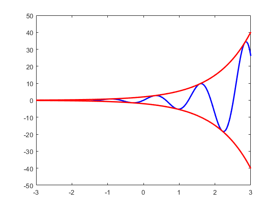
In this previous example, we can get a fairly good idea of how to sketch out the graph of this function. Since \(\sin(2x)\) oscillates between \(-1\) and \(1\text{,}\) the graph of \(y = 5e^{3x}\sin(2x)\) will oscillate between the graphs of \(5e^{3x}\) and \(-5e^{3x}\text{.}\) These curves that surround the graph of the solution are called envelope curves for the solution. In Figure 2.2.10, this phenomenon is illustrated for the function \(y = 2e^x\sin(5x)\text{.}\)
This is simple when there is only one term in the function we want to draw. When both sine and cosine terms appear, this can get more tricky, but we can still work it out. In the more general case, the solution will look something like
\begin{equation*}
y = Ae^{\alpha x}\cos(\beta x) + B e^{\alpha x} \sin(\beta x).
\end{equation*}
We can first factor out an \(e^{\alpha x}\text{,}\) and then we want to write \(A \cos(\beta x) + B \sin(\beta x)\) as a single trigonometric function. The identity we want to use here is the trigonometric identity
If there is an angle \(\delta\) so that \(A = \cos(\delta)\) and \(B = \sin(\delta)\text{,}\) then we could write
\begin{equation*}
A \cos(\beta x) + B \sin(\beta x) = \cos(\beta x - \delta)
\end{equation*}
and we would be done. However, this does not always happen; the main issue being that \(\cos^2(\delta) + \sin^2(\delta) = 1\) for all \(\delta\text{,}\) but it is not necessarily the case that \(A^2 + B^2 = 1\text{.}\) But we can force this last condition. If we define \(R = \sqrt{A^2 + B^2}\text{,}\) then we can rewrite this expression as
\begin{align*}
A \cos(\beta x) + B \sin(\beta x) \amp= R \left( \frac{A}{\sqrt{A^2 + B^2}} \cos(\beta x) + \frac{B}{\sqrt{A^2 + B^2}}\sin(\beta x)\right) \\
\amp= R \left( \cos(\delta) \cos(\beta x) + \sin(\delta) \sin(\beta x) \right) \\
\amp= R \cos(\beta x - \delta)
\end{align*}
Note that in order to determine these envelope curves, you do not need to determine the \(\delta\) value in the representation of the solution. All you need is the value of \(R\text{,}\) which can be computed as \(\sqrt{A^2 + B^2}\) where \(A\) and \(B\) are the coefficients of the sine and cosine terms in the solution.
We solve the initial value problem by normal techniques from this section. The characteristic equation is \(r^2 + 2r + 5 = 0\text{,}\) which has roots \(r = -1 \pm 2i\text{.}\) Therefore, the general solution of the differential equation is
\begin{equation*}
y = C_1e^{-x}\cos(2x) + C_2 e^{-x}\sin(2x).
\end{equation*}
Plugging in \(0\) gives that \(y(0) = 1 = C_1\text{,}\) and the derivative of this general solution is
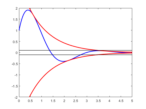
In order to find this threshold \(T\) where the solution will stay within \(0.1\) of zero, we need to figure out when this envelope curves get to the \(0.1\) threshold. Once the envelope curves get to that level, we know that the full solution must be trapped there as well. We can solve
So, for all values of \(x\) larger than 3.454, the solution will be within \(0.1\) of zero. This is illustrated in Figure 2.2.12. Note that we did not find the best value \(T\) here, as it probably could be made smaller using the actual solution. The issue here is that because the solution is oscillating, it may end up staying inside the \(0.1\) cutoff before that value of time, but this is the lowest value of \(T\) that we can prove and validate using envelope curves.
Figure2.2.12.Plot of the function \(e^{-x}\cos(2x) + 3e^{-x}\sin(2x)\) with envelope curves illustrating the bounds on the function for large values of \(x\text{.}\)
Let us revisit the Cauchy-Euler equations of Exercise Group 24–25. Suppose now that \({(b-a)}^2-4ac < 0\text{.}\) Find a formula for the general solution of \(a x^2 y'' + b x y' + c y = 0\text{.}\) Hint: Note that \(x^r = e^{r \ln x}\text{.}\)
Find a second order, constant coefficient differential equation with general solution given by \(y(t) = C_1e^{x} \cos(2x) + C_2e^{2x}\sin(x)\) or explain why there is no such thing.
There is no such equation. The two roots will always be complex conjugates, which means the exponential parts will match, and the trigonometric functions will have the same argument.
Find a second order, constant coefficient differential equation with general solution given by \(y(t) = C_1e^{x} \cos(2x) + C_2e^{x}\sin(2x)\) or explain why there is no such thing.