Bifurcation diagrams

Section 1.8 Bifurcation diagrams

Objectives

After this section, you will be able to:

Draw and analyze bifurcation diagrams for autonomous equations with parameter.
🔗

🔗

An extension of the topic of autonomous equation is autonomous equations with parameter. The idea is that we have a differential equation that has no explicit dependence on time, but does have a dependence on an outside parameter, which is a constant set by the physical situation. In terms of physical problems, this parameter will tend to be something that we can adjust to change how the differential equation behaves. For example, in a logistic differential equation

\begin{equation*} \frac{dx}{dt} = ax(K-x) \end{equation*}

either the \(a\) or the \(K\) (or both) could be adjustable parameters. For a given value of the parameter, the differential equation behaves like a standard autonomous differential equation, but we can get different properties of this equation for different values of the parameter.

🔗

Definition 1.8.1.

An autonomous equation with parameter \(\alpha\) is a differential equation of the form

\begin{equation*} \frac{dx}{dt} = f_\alpha(x) \end{equation*}

where, for every value of \(\alpha\text{,}\) \(f_\alpha(x)\) is a function of the single variable \(x\text{.}\)

🔗

Later, we will want to view \(f_\alpha(x)\) as a two-variable function of \(x\) and \(\alpha\text{,}\) but for now, we want to think about it as a function of just \(x\) for a fixed value of \(\alpha\text{.}\) We want to be able to analyze what happens to this equation for different values of \(\alpha\text{.}\) Since it is an autonomous equation, we can do this using phase lines. This will be easiest to see through an example.

🔗

Example 1.8.2. .

Consider the differential equation

\begin{equation*} \frac{dx}{dt} = x(x^2 - \alpha), \end{equation*}

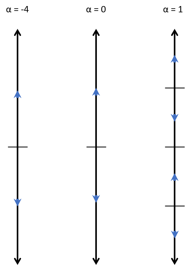
which fits the description of an autonomous equation with parameter \(\alpha\text{.}\) Describe what happens in this differential equation for \(\alpha = -4\text{,}\) \(\alpha = 0\text{,}\) and \(\alpha = 1\text{.}\)

🔗

Solution.

We can draw a phase line for \(\alpha = -4\text{,}\) \(\alpha = 0\) and \(\alpha = 1\text{.}\)

🔗

ALT TEXT HERE — Figure 1.8.3. Phase lines for the differential equation \(\frac{dx}{dt} = x(x^2 - \alpha)\) for \(\alpha = -4,\ 0,\ 1\text{.}\)
🔗

It is clear that something happens with this equation between \(\alpha = -4\) and \(\alpha = 1\text{.}\) We go from having only one equilibrium solution at \(\alpha = -4\) to having three equilibrium solutions at \(\alpha = 1\text{.}\) In addition, the solution at \(y=0\) is unstable for \(\alpha = -4\text{,}\) while it is asymptotically stable for \(\alpha = 1\text{.}\) If we want to figure out when this change happens, we’ll need a better way to analyze this problem.

🔗

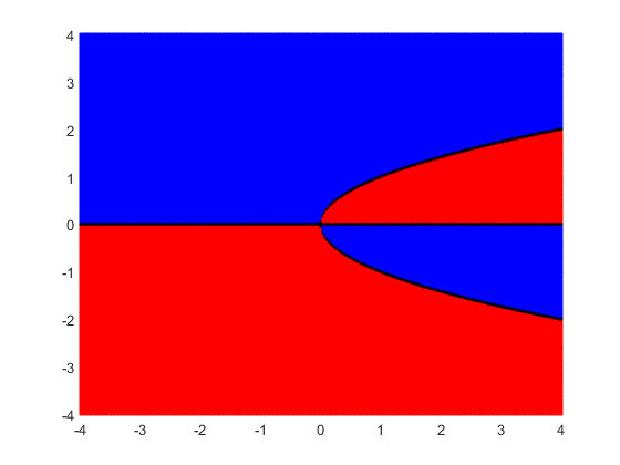
How can we better approach this problem? The idea is to think about when the solution to the differential equation will be increasing or decreasing as a function of the two variables \(\alpha\) and \(x\text{.}\) Based on the structure of the differential equation, the solution will be increasing when the function \(f_\alpha(x)\) is positive and will be decreasing when \(f_\alpha(x)\) is negative. Since a phase line is a plot of this information for a given value of \(\alpha\text{,}\) we essentially want to plot all of these phase lines on a two-dimensional graph. This graph is called a bifurcation diagram. Figure 1.8.4 shows a bifurcation diagram for the example \(\frac{dx}{dt} = x(x^2-\alpha)\text{.}\)

🔗

Within this picture, we can see all of our phase lines from before, because at any value of \(\alpha\text{,}\) taking the vertical slice of this graph at that value, we get the phase line. If we want to consider \(\alpha = -4\text{,}\) then we can look above the horizontal coordinate \(-4\text{,}\) and that will give us the phase line for \(\alpha = -4\text{.}\) The same goes for any other value of \(\alpha\) we want to consider. For instance, we can also see that for any \(\alpha \leq 0\text{,}\) there will be one equilibrium solution, and for \(\alpha > 0\) there are three equilibrium solutions, indicated by the three black curves above each of those \(\alpha\) values.

🔗

From this, we can see that the point at which the behavior changes is \(\alpha = 0\text{.}\) Thus, for this problem \(\alpha = 0\) is called the bifurcation point. This is defined to be the value of the parameter for which the overall behavior of the equation changes. This can be a change in the number of equilibrium solutions, the stability of these equilibrium solutions, or both. For this particular example, we have both of these. We go from 1 equilibrium solution to 3, and the solution at \(y=0\) changes in stability. This type of bifurcation is called a “pitchfork bifurcation” based on the shape of the equilibrium solutions near the bifurcation point.

🔗

Another example of a bifurcation of a different form can be seen in the example of the logistic equation with harvesting. Suppose an alien race really likes to eat humans. They keep a planet with humans on it and harvest the humans at a rate of \(h\) million humans per year. Suppose \(x\) is the number of humans in millions on the planet and \(t\) is time in years. Let \(M\) be the limiting population when no harvesting is done. The number \(k > 0\) is a constant depending on how fast humans multiply. Our equation becomes

\begin{equation*} \frac{dx}{dt} = kx(M-x) - h . \end{equation*}

In this setup, M and k are fixed values, and the parameter that is being adjusted for this equation is \(h\text{.}\) We expand the right-hand side and set it to zero.

\begin{equation*} kx(M-x) - h = -kx^2+kMx - h = 0. \end{equation*}

Solving for the critical points using the quadratic formula, let us call them \(A\) and \(B\text{,}\) we get

\begin{equation*} A = \frac{kM + \sqrt{{(kM)}^2 - 4hk}}{2k}, \qquad B = \frac{kM - \sqrt{{(kM)}^2 - 4hk}}{2k} . \end{equation*}

🔗

Checkpoint 1.8.5.

Sketch a phase diagram for different possibilities. Note that these possibilities are \(A > B\text{,}\) or \(A=B\text{,}\) or \(A\) and \(B\) both complex (i.e. no real solutions). Hint: Fix some simple \(k\) and \(M\) and then vary \(h\text{.}\)

🔗

Example 1.8.6.

For example, let \(M=8\) and \(k=0.1\text{.}\) What happens for different values of \(h\) in this situation?

🔗

Solution.

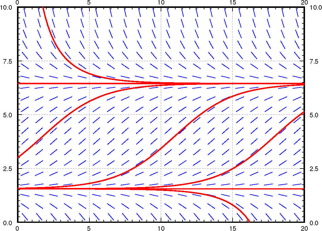
When \(h=1\text{,}\) then \(A\) and \(B\) are distinct and positive. The slope field we get is in Figure 1.8.7 . As long as the population starts above \(B\text{,}\) which is approximately 1.55 million, then the population will not die out. It will in fact tend towards \(A \approx 6.45\) million. If ever some catastrophe happens and the population drops below \(B\text{,}\) humans will die out, and the fast food restaurant serving them will go out of business.

🔗

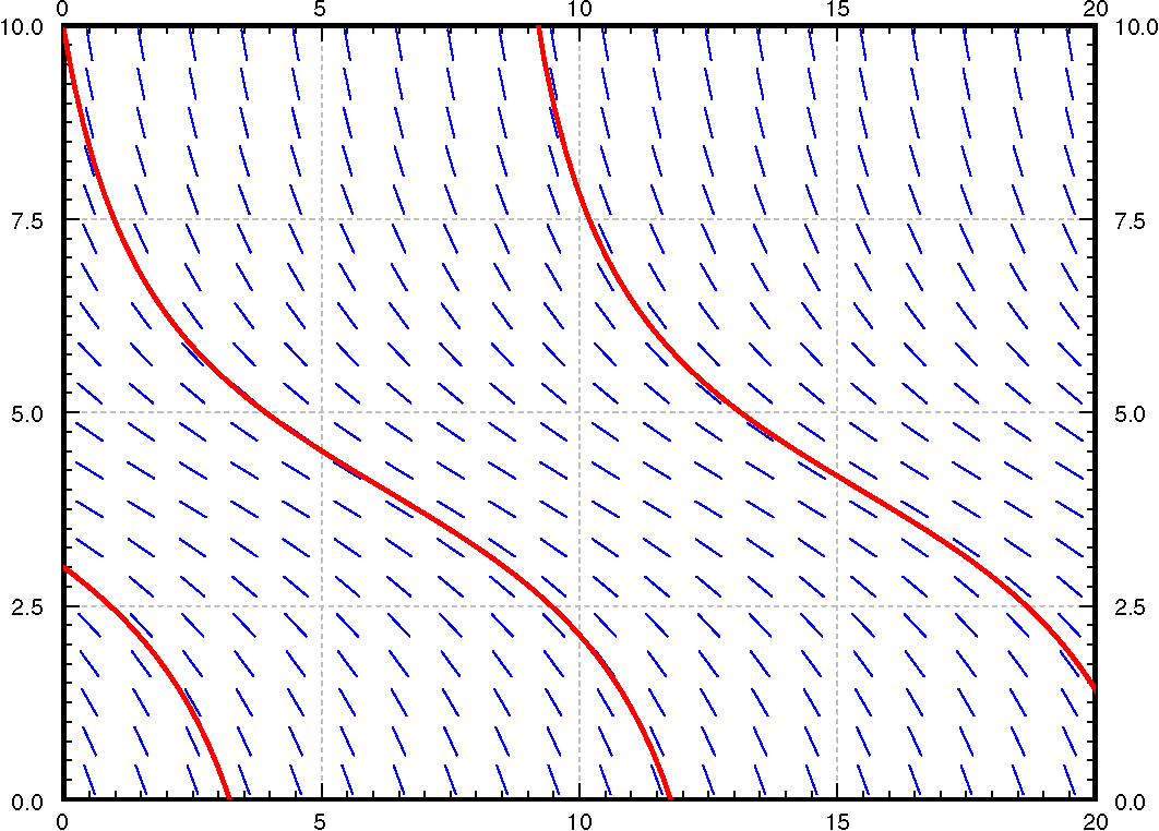
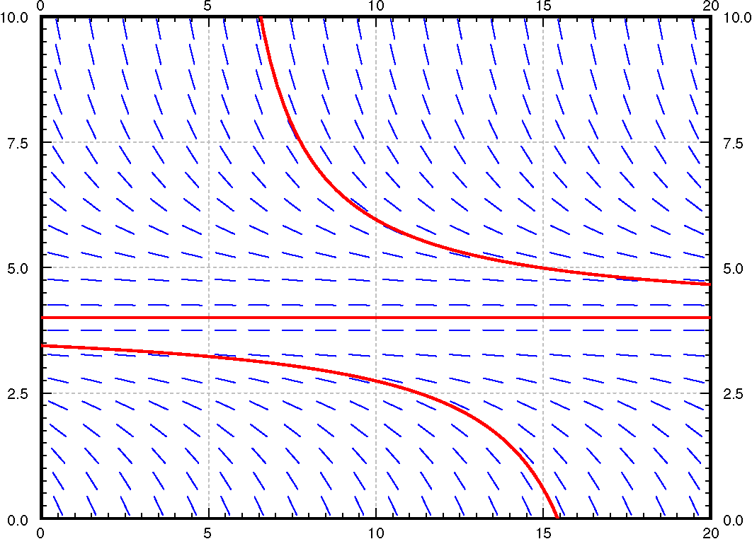
When \(h = 1.6\text{,}\) then \(A=B=4\text{.}\) There is only one critical point and it is semistable. When the population starts above 4 million it will tend towards 4 million. If it ever drops below 4 million, humans will die out on the planet. This scenario is not one that we (as the human fast food proprietor) want to be in. A small perturbation of the equilibrium state and we are out of business. There is no room for error. See Figure 1.8.8.

🔗

Finally if we are harvesting at 2 million humans per year, there are no critical points. The population will always plummet towards zero, no matter how well stocked the planet starts. See Figure 1.8.9.

🔗

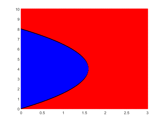
All of these can also be seen from the bifurcation diagram, which is drawn in Figure 1.8.10. The values \(A\) and \(B\) discussed above represent the upper and lower branches of the parabola in the figure. For any \(h > 1.6\text{,}\) there are no equilibrium solutions and the phase line is entirely decreasing, meaning the solution will converge to zero no matter what. For \(h < 1.6\text{,}\) there are two equilibrium solutions, with the top one asymptotically stable and the bottom one unstable. At \(h=1.6\) is where the bifurcation point occurs for this example. This is an example of a “saddle-node” bifurcation, as the two equilibrium solutions collide with each other at the bifurcation point and disappear.

🔗

Another way to visualize this situation is by plotting the function \(f_\alpha(x)\) for the different values of \(\alpha\text{.}\) The places where this function is zero give the equilibrium solutions, and we can determine bifurcation values by looking for where the zeros of this function change behavior. For this particular example, the graphs of \(f_\alpha(x)\) are drawn in Figure 1.8.11.

🔗

The values of \(\alpha\) we are looking for are those where the number and types of zeros change for the function \(f_\alpha(x)\text{.}\) In this figure, we see that for \(\alpha < 1.6\text{,}\) the parabola crosses the \(x\) axis twice, resulting in two zeros and two equilibrium solutions. For \(\alpha = 1.6\text{,}\) there is one (double) root, and for \(\alpha > 1.6\text{,}\) there are no equilibrium solutions, and the function \(f_\alpha(x)\) is always negative. Since the number of roots/zeros changes at \(\alpha = 1.6\text{,}\) that means that \(1.6\) is the bifurcation point for this equation. We can also see this from the equation, since the equilibrium solutions are determined by the values of \(x\) where

\begin{equation*} 0.1x(8-x) - \alpha = 0 \qquad \text{ or } \qquad -0.1x^2 + 0.8x - \alpha = 0 \end{equation*}

which can be found by the quadratic formula

\begin{equation*} x = \frac{0.8 \pm \sqrt{0.64 - 4(0.1)(\alpha)}}{0.2}. \end{equation*}

Roots to this equation do not exist (because they are complex) if \(0.64 - 0.4\alpha < 0\text{,}\) or \(\alpha > 1.6\text{.}\)

🔗

Exercises Exercises

1.

Start with the logistic equation \(\frac{dx}{dt} = kx(M-x)\text{.}\) Suppose we modify our harvesting. That is we will only harvest an amount proportional to current population. In other words, we harvest \(hx\) per unit of time for some \(h > 0\) (Similar to earlier example with \(h\) replaced with \(hx\)).

🔗

(a)

Construct the differential equation.

🔗

Answer.

\(\frac{dx}{dt} = kx\left(\frac{Mk-h}{k} - x\right)\)

🔗

(b)

Show that if \(kM > h\text{,}\) then the equation is still logistic.

🔗

Answer.

It changes the effective M

🔗

(c)

What happens when \(kM < h\text{?}\)

🔗

Answer.

Population always decreases.

🔗

2.

Assume that a population of fish in a lake satisfies \(\frac{dx}{dt} = kx(M-x)\text{.}\) Now suppose that fish are continually added at \(A\) fish per unit of time.

🔗